Time Series

6.7. Time Series#

This section shows some tools to work with datetime and time series.

6.7.1. Extract Dates from Text with Datefinder#

Extracting dates from unstructured text can be challenging and time-consuming, especially when the format of the dates varies significantly within the same text:

# Example Input
string_with_dates = """
We have one meeting on May 17th, 2021 at 9:00am 
and another meeting on 5/18/2021 at 10:00. 
I hope you can attend one of the meetings.
"""

# Traditional string processing to find dates
import re

# Basic regex for dates
pattern = r"(\b\d{1,2}/\d{1,2}/\d{4}\b)|(\b\w+\s\d{1,2}(st|nd|rd|th)?,\s\d{4}\b)"
matches = re.findall(pattern, string_with_dates)
print(
    f"Matches: {[match[0] or match[1] for match in matches]}"
)  # Limited and inflexible

Matches: ['May 17th, 2021', '5/18/2021']

Datefinder simplifies the process of identifying and extracting dates from text, even when the formats vary:

import datefinder

# Example Input
string_with_dates = """
We have one meeting on May 17th, 2021 at 9:00am 
and another meeting on 5/18/2021 at 10:00. 
I hope you can attend one of the meetings.
"""

# Extract dates from text
matches = datefinder.find_dates(string_with_dates)

## Print each match
for match in matches:
    print(match)

import datefinder

# Example Input
string_with_dates = """
We have one meeting on May 17th, 2021 at 9:00am 
and another meeting on 5/18/2021 at 10:00. 
I hope you can attend one of the meetings.
"""

## Extract dates from text
matches = datefinder.find_dates(string_with_dates)

## Print each match
for match in matches:
    print(match)

2021-05-17 09:00:00
2021-05-18 10:00:00

In the above code:

datefinder.find_dates() - This function identifies potential date strings in the input text and converts them into datetime objects.
string_with_dates - Text containing dates in multiple formats.
matches - An iterator returning each located date as a datetime object.

Link to Datefinder.

6.7.2. Fastai’s add_datepart: Add Relevant DateTime Features in One Line of Code#

Time series analysis often benefits from date-based features like year, month, and day of week. Fastai’s add_datepart method generates these features in one line of code, simplifying data preparation.

from datetime import datetime

import pandas as pd
from fastai.tabular.core import add_datepart

df = pd.DataFrame(
    {
        "date": [
            datetime(2020, 2, 5),
            datetime(2020, 2, 6),
            datetime(2020, 2, 7),
            datetime(2020, 2, 8),
        ],
        "val": [1, 2, 3, 4],
    }
)

df

	date	val
0	2020-02-05	1
1	2020-02-06	2
2	2020-02-07	3
3	2020-02-08	4

df = add_datepart(df, "date")
df.columns

Index(['val', 'Year', 'Month', 'Week', 'Day', 'Dayofweek', 'Dayofyear',
       'Is_month_end', 'Is_month_start', 'Is_quarter_end', 'Is_quarter_start',
       'Is_year_end', 'Is_year_start', 'Elapsed'],
      dtype='object')

Link to Fastai’s methods to work with tabular data

6.7.3. Maya: Convert the string to datetime automatically#

Date string conversion to datetime can be tedious using strptime(). The maya library simplifies this process by automatically parsing date strings without needing to specify the format.

import maya

## Automatically parse datetime string
string = "2016-12-16 18:23:45.423992+00:00"
maya.parse(string).datetime()

datetime.datetime(2016, 12, 16, 18, 23, 45, 423992, tzinfo=<UTC>)

Better yet, if you want to convert the string to a different time zone (for example, CST), you can parse that into maya’s datetime function.

maya.parse(string).datetime(to_timezone="US/Central")

datetime.datetime(2016, 12, 16, 12, 23, 45, 423992, tzinfo=<DstTzInfo 'US/Central' CST-1 day, 18:00:00 STD>)

Link to maya.

6.7.4. Pendulum: Python Datetimes Made Easy#

While native datetime instances are sufficient for simple cases, they can become difficult to work with when dealing with more complex scenarios.

Conversely, Pendulum offers a more intuitive and user-friendly API, making it a convenient drop-in replacement for the standard datetime class.

The examples below demonstrate the syntax differences between using the standard datetime library and Pendulum.

Datetime:

from datetime import datetime, timedelta

import pytz

## Creating a datetime
now = datetime.now()
print(f"Current time: {now}")

## Date arithmetic
future = now + timedelta(days=7)
print(f"7 days from now: {future}")

## Timezone handling
utc_now = datetime.now(pytz.UTC)
tokyo_tz = pytz.timezone("Asia/Tokyo")
tokyo_time = utc_now.astimezone(tokyo_tz)
print(f"Time in Tokyo: {tokyo_time}")

## Parsing (requires exact format)
parsed = datetime.strptime("2023-05-15 14:30:00", "%Y-%m-%d %H:%M:%S")

## Time difference (not human-readable)
diff = parsed - now
print(f"Difference: {diff}")

Current time: 2024-09-02 19:18:13.589774
7 days from now: 2024-09-09 19:18:13.589774
Time in Tokyo: 2024-09-03 09:18:13.590063+09:00
Difference: -477 days, 19:11:46.410226

Pendulum:

import pendulum

## Creating a datetime
now = pendulum.now()
print(f"Current time: {now}")

## Date arithmetic (more intuitive than datetime)
future = now.add(days=7)
print(f"7 days from now: {future}")

## Timezone handling
tokyo_time = now.in_timezone("Asia/Tokyo")
print(f"Time in Tokyo: {tokyo_time}")

## Parsing without specifying format
parsed = pendulum.parse("2023-05-15 14:30:00")
print(f"Parsed date: {parsed}")

## Human-readable differences
diff = parsed - now
print(f"Difference: {diff.in_words()}")

Current time: 2024-09-02 18:58:20.467988-05:00
7 days from now: 2024-09-09 18:58:20.467988-05:00
Time in Tokyo: 2024-09-03 08:58:20.467988+09:00
Parsed date: 2023-05-15 14:30:00+00:00
Difference: -1 year -3 months -2 weeks -4 days -9 hours -28 minutes -20 seconds

Link to Pendulum.

6.7.5. traces: A Python Library for Unevenly-Spaced Time Series Analysis#

To analyze unevenly-spaced time series, you can use the traces library. It allows you to infer missing values in your time series based on the data you already have.

Here’s an example where we log working hours for several dates but miss a few:

## Log working hours for each date
from datetime import datetime

import traces

working_hours = traces.TimeSeries()
working_hours[datetime(2021, 9, 10)] = 10
working_hours[datetime(2021, 9, 12)] = 5
working_hours[datetime(2021, 9, 13)] = 6
working_hours[datetime(2021, 9, 16)] = 2

To retrieve the hours for dates where no data was logged, traces fills in the gaps using neighboring values:

## Get value on 2021/09/11
working_hours[datetime(2021, 9, 11)]

## Get value on 2021/09/14
working_hours[datetime(2021, 9, 14)]

You can also calculate the distribution of working hours over a range of dates:

distribution = working_hours.distribution(
    start=datetime(2021, 9, 10), end=datetime(2021, 9, 16)
)
distribution

Histogram({5: 0.16666666666666666, 6: 0.5, 10: 0.3333333333333333})

From this, we can infer that 50% of the time, 6 hours were logged per day.

To get the median and mean working hours across the range:

distribution.median()

6.0

distribution.mean()

7.166666666666666

Link to traces

6.7.6. Extract holiday from date column#

To identify holidays from a date, use the holidays package. This package offers a dictionary of holidays for various countries.

The following code checks if “2020-07-04” is a US holiday and retrieves its name:

from datetime import date

import holidays

us_holidays = holidays.UnitedStates()

"2014-07-04" in us_holidays

True

The package handles various date formats:

us_holidays.get("2014-7-4")

'Independence Day'

us_holidays.get("2014/7/4")

'Independence Day'

Link to holidays.

6.7.7. Workalendar: Handle Working-Day Computation in Python#

To manage calendars, holidays, and working-day computations, use the workalendar package. It supports nearly 100 countries worldwide.

from datetime import date

from workalendar.asia import Japan
from workalendar.usa import UnitedStates

## Get all holidays in the US

US_cal = UnitedStates()
US_cal.holidays(2024)

[(datetime.date(2024, 1, 1), 'New year'),
 (datetime.date(2024, 1, 15), 'Birthday of Martin Luther King, Jr.'),
 (datetime.date(2024, 2, 19), "Washington's Birthday"),
 (datetime.date(2024, 5, 27), 'Memorial Day'),
 (datetime.date(2024, 7, 4), 'Independence Day'),
 (datetime.date(2024, 9, 2), 'Labor Day'),
 (datetime.date(2024, 10, 14), 'Columbus Day'),
 (datetime.date(2024, 11, 11), 'Veterans Day'),
 (datetime.date(2024, 11, 28), 'Thanksgiving Day'),
 (datetime.date(2024, 12, 25), 'Christmas Day')]

US_cal.is_working_day(date(2024, 9, 15))  # Sunday

False

US_cal.is_working_day(date(2024, 9, 2))  # Labor Day

False

## Calculate working days between 2024/1/19 and 2024/5/15
US_cal.get_working_days_delta(date(2024, 1, 19), date(2024, 5, 15))

## Get holidays in Japan
JA_cal = Japan()
JA_cal.holidays(2024)

[(datetime.date(2024, 1, 1), 'New year'),
 (datetime.date(2024, 1, 8), 'Coming of Age Day'),
 (datetime.date(2024, 2, 11), 'Foundation Day'),
 (datetime.date(2024, 2, 23), "The Emperor's Birthday"),
 (datetime.date(2024, 3, 20), 'Vernal Equinox Day'),
 (datetime.date(2024, 4, 29), 'Showa Day'),
 (datetime.date(2024, 5, 3), 'Constitution Memorial Day'),
 (datetime.date(2024, 5, 4), 'Greenery Day'),
 (datetime.date(2024, 5, 5), "Children's Day"),
 (datetime.date(2024, 7, 15), 'Marine Day'),
 (datetime.date(2024, 8, 11), 'Mountain Day'),
 (datetime.date(2024, 9, 16), 'Respect-for-the-Aged Day'),
 (datetime.date(2024, 9, 22), 'Autumnal Equinox Day'),
 (datetime.date(2024, 10, 14), 'Sports Day'),
 (datetime.date(2024, 11, 3), 'Culture Day'),
 (datetime.date(2024, 11, 23), 'Labour Thanksgiving Day')]

Link to Workalendar.

6.7.8. Pmdarima: Harness R’s auto.arima Power with a scikit-learn-Like Interface#

To achieve functionality similar to R’s auto.arima within a scikit-learn-like interface, use Pmdarima.

import matplotlib.pyplot as plt
import numpy as np
import pmdarima as pm
from pmdarima.model_selection import train_test_split

## Load/split your data
y = pm.datasets.load_wineind()
train, test = train_test_split(y, train_size=150)

## Fit your model
model = pm.auto_arima(train, seasonal=True, m=12)

## Make your forecasts
forecasts = model.predict(test.shape[0])  # predict N steps into the future

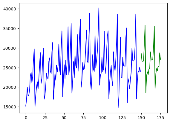
## Visualize the forecasts (blue=train, green=forecasts)
x = np.arange(y.shape[0])
plt.plot(x[:150], train, c="blue")
plt.plot(x[150:], forecasts, c="green")
plt.show()

../_images/42fb2ec7417b566b4429c81126325a619d2f15a982fbd8f57f42399a735e81f8.png

Fitting a more complex pipeline on the sunspots dataset, serializing it, and then loading it from disk to make predictions:

import pickle

import pmdarima as pm
from pmdarima.model_selection import train_test_split
from pmdarima.pipeline import Pipeline
from pmdarima.preprocessing import BoxCoxEndogTransformer

## Load/split your data
y = pm.datasets.load_sunspots()
train, test = train_test_split(y, train_size=2700)

## Define and fit your pipeline
pipeline = Pipeline(
    [
        ("boxcox", BoxCoxEndogTransformer(lmbda2=1e-6)),
        (
            "arima",
            pm.AutoARIMA(seasonal=True, m=12, suppress_warnings=True, trace=True),
        ),
    ]
)

pipeline.fit(train)

# Serialize your model just like you would in scikit:
with open("model.pkl", "wb") as pkl:
    pickle.dump(pipeline, pkl)

## Load it and make predictions seamlessly:
with open("model.pkl", "rb") as pkl:
    mod = pickle.load(pkl)
    print(mod.predict(15))

Performing stepwise search to minimize aic
 ARIMA(2,1,2)(1,0,1)[12] intercept   : AIC=inf, Time=6.52 sec
 ARIMA(0,1,0)(0,0,0)[12] intercept   : AIC=10383.210, Time=0.04 sec
 ARIMA(1,1,0)(1,0,0)[12] intercept   : AIC=10020.218, Time=0.80 sec
 ARIMA(0,1,1)(0,0,1)[12] intercept   : AIC=9831.422, Time=1.11 sec
 ARIMA(0,1,0)(0,0,0)[12]             : AIC=10381.212, Time=0.05 sec
 ARIMA(0,1,1)(0,0,0)[12] intercept   : AIC=9830.357, Time=0.12 sec
 ARIMA(0,1,1)(1,0,0)[12] intercept   : AIC=9831.459, Time=0.70 sec
 ARIMA(0,1,1)(1,0,1)[12] intercept   : AIC=9831.930, Time=3.67 sec
 ARIMA(1,1,1)(0,0,0)[12] intercept   : AIC=9817.480, Time=0.22 sec
 ARIMA(1,1,1)(1,0,0)[12] intercept   : AIC=9817.508, Time=1.15 sec
 ARIMA(1,1,1)(0,0,1)[12] intercept   : AIC=9817.413, Time=2.34 sec
 ARIMA(1,1,1)(1,0,1)[12] intercept   : AIC=9817.657, Time=3.29 sec
 ARIMA(1,1,1)(0,0,2)[12] intercept   : AIC=9817.996, Time=4.25 sec
 ARIMA(1,1,1)(1,0,2)[12] intercept   : AIC=9820.047, Time=4.23 sec
 ARIMA(1,1,0)(0,0,1)[12] intercept   : AIC=10020.213, Time=0.82 sec
 ARIMA(2,1,1)(0,0,1)[12] intercept   : AIC=9817.896, Time=2.30 sec
 ARIMA(1,1,2)(0,0,1)[12] intercept   : AIC=9818.625, Time=2.49 sec
 ARIMA(0,1,0)(0,0,1)[12] intercept   : AIC=10385.194, Time=0.98 sec
 ARIMA(0,1,2)(0,0,1)[12] intercept   : AIC=9816.628, Time=1.55 sec
 ARIMA(0,1,2)(0,0,0)[12] intercept   : AIC=9816.710, Time=0.41 sec
 ARIMA(0,1,2)(1,0,1)[12] intercept   : AIC=9816.881, Time=4.06 sec
 ARIMA(0,1,2)(0,0,2)[12] intercept   : AIC=9817.222, Time=3.11 sec
 ARIMA(0,1,2)(1,0,0)[12] intercept   : AIC=9816.722, Time=1.20 sec
 ARIMA(0,1,2)(1,0,2)[12] intercept   : AIC=9813.247, Time=10.18 sec
 ARIMA(0,1,2)(2,0,2)[12] intercept   : AIC=inf, Time=19.62 sec
 ARIMA(0,1,2)(2,0,1)[12] intercept   : AIC=9819.401, Time=3.04 sec
 ARIMA(0,1,1)(1,0,2)[12] intercept   : AIC=9834.327, Time=3.96 sec
 ARIMA(1,1,2)(1,0,2)[12] intercept   : AIC=9815.242, Time=17.06 sec
 ARIMA(0,1,3)(1,0,2)[12] intercept   : AIC=9815.236, Time=15.52 sec
 ARIMA(1,1,3)(1,0,2)[12] intercept   : AIC=9816.564, Time=23.76 sec
 ARIMA(0,1,2)(1,0,2)[12]             : AIC=9811.253, Time=6.00 sec
 ARIMA(0,1,2)(0,0,2)[12]             : AIC=9815.230, Time=1.26 sec
 ARIMA(0,1,2)(1,0,1)[12]             : AIC=9814.890, Time=1.09 sec
 ARIMA(0,1,2)(2,0,2)[12]             : AIC=inf, Time=9.39 sec
 ARIMA(0,1,2)(0,0,1)[12]             : AIC=9814.636, Time=0.61 sec
 ARIMA(0,1,2)(2,0,1)[12]             : AIC=9817.409, Time=1.12 sec
 ARIMA(0,1,1)(1,0,2)[12]             : AIC=9832.334, Time=1.30 sec
 ARIMA(1,1,2)(1,0,2)[12]             : AIC=9813.248, Time=5.01 sec
 ARIMA(0,1,3)(1,0,2)[12]             : AIC=9813.242, Time=4.11 sec
 ARIMA(1,1,1)(1,0,2)[12]             : AIC=9818.055, Time=1.73 sec
 ARIMA(1,1,3)(1,0,2)[12]             : AIC=9814.546, Time=8.53 sec

Best model:  ARIMA(0,1,2)(1,0,2)[12]          
Total fit time: 178.878 seconds
[26.73630214 26.72738664 27.33806937 27.97670263 26.94336951 27.27600697
 26.76335004 27.06207145 28.18910652 27.76778119 28.01474934 27.41947969
 27.57286429 27.30950555 27.63971231]

Link to Pmdarima.

6.7.9. aeon: The Ultimate Library for Time-Series Forecasting and Classification#

aeon is a library for time-series data that is compatible with scikit-learn and offers a variety of advanced algorithms for learning tasks like forecasting and classification.

import pandas as pd
from aeon.forecasting.trend import TrendForecaster

y = pd.Series([20.0, 40.0, 60.0, 80.0, 100.0])
forecaster = TrendForecaster()

# fit the forecaster
forecaster.fit(y)

# forecast the next 3 values
forecaster.predict(fh=[1, 2, 3])

  120.0
  140.0
  160.0
dtype: float64

import numpy as np
from aeon.classification.distance_based import KNeighborsTimeSeriesClassifier

# 3 samples and 6 time steps
X = np.array([[1, 2, 3, 4, 5, 5], [1, 2, 3, 4, 4, 2], [8, 7, 6, 5, 4, 4]])

# class labels for each sample
y = np.array(["low", "low", "high"])

## Define the classifier
clf = KNeighborsTimeSeriesClassifier(distance="dtw")

# fit the classifier on train data
clf.fit(X, y)

## Test data
X_test = np.array([[2, 2, 2, 2, 2, 2], [6, 6, 6, 6, 6, 6]])

## Make class predictions on new data
y_pred = clf.predict(X_test)
y_pred

array(['low', 'high'], dtype='<U4')

Link to aeon.

6.7.10. Ruptures: Detecting Change Points in Non-Stationary Signals#

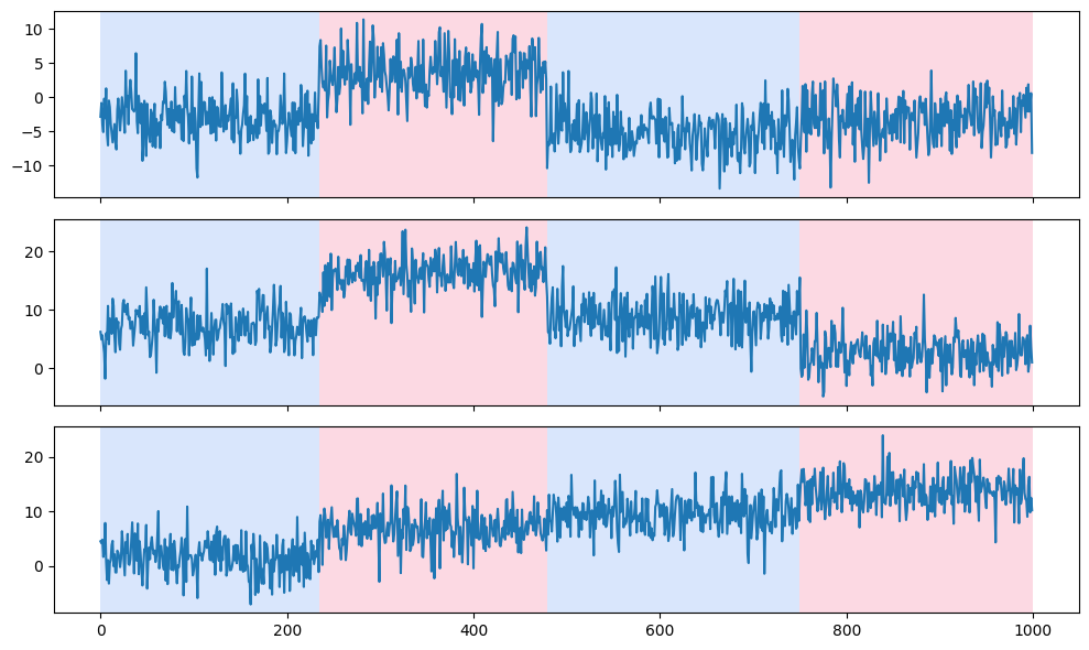
Use ruptures to detect change points from non-stationary signals such as trend, seasonality, and variance.

With change points, you can detect anomalies or deviations from the expected behavior and gain insights into when these transitions occur.

import matplotlib.pyplot as plt
import ruptures as rpt

# generate signal
n_samples, n_features, sigma = 1000, 3, 3
num_breakpoints = 3
signal, true_breakpoints = rpt.pw_constant(
    n_samples, n_features, num_breakpoints, noise_std=sigma
)

# detection
algo = rpt.Pelt(model="rbf").fit(signal)
predicted_breakpoints = algo.predict(pen=10)

# display
rpt.display(signal, predicted_breakpoints)
plt.show()

../_images/1030df48742b5c76a98e591fa5c6c6af542119e8fdedbb53ae82d6daec4163cc.png

Link to ruptures.

6.7.11. GluonTS: Probabilistic Time Series Modeling in Python#

Probabilistic models offer a range of possible future outcomes, rather than a single fixed prediction, allowing for the assessment of risk associated with adverse events.

GluonTS streamlines the process of using probabilistic models for time series data.

import pandas as pd
import matplotlib.pyplot as plt

from gluonts.dataset.pandas import PandasDataset
from gluonts.dataset.split import split
from gluonts.torch import DeepAREstimator

## Load data from a CSV file into a PandasDataset
df = pd.read_csv(
    "https://raw.githubusercontent.com/AileenNielsen/"
    "TimeSeriesAnalysisWithPython/master/data/AirPassengers.csv",
    index_col=0,
    parse_dates=True,
)
dataset = PandasDataset(df, target="#Passengers")

## Split the data for training and testing
training_data, test_gen = split(dataset, offset=-36)
test_data = test_gen.generate_instances(prediction_length=12, windows=3)

## Train the model and make predictions
model = DeepAREstimator(
    prediction_length=12, freq="M", trainer_kwargs={"max_epochs": 5}
).train(training_data)

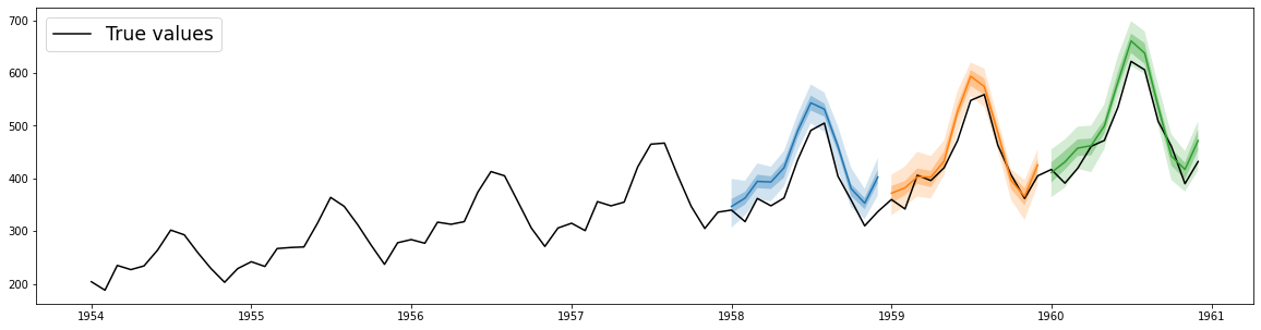
forecasts = list(model.predict(test_data.input))

## Plot predictions
plt.plot(df["1954":], color="black")
for forecast in forecasts:
  forecast.plot()
plt.legend(["True values"], loc="upper left", fontsize="xx-large")
plt.show()

Link to GluonTS.

6.7.12. tfcausalimpact: Understand Causal Relationships in Time Series Data#

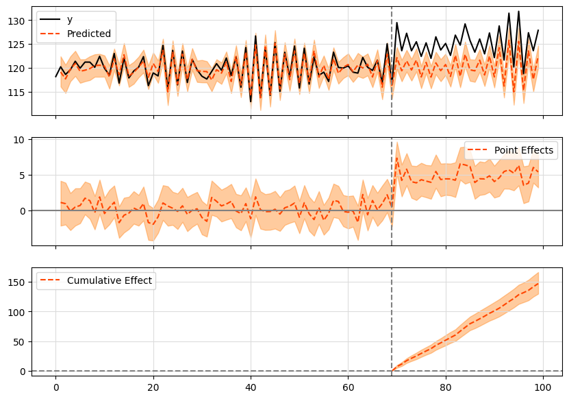
You’re running a marketing campaign and see a user increase. But how do you know if it’s due to the campaign or just a coincidence?

That is when tfcausalimpact comes in handy. It forecasts future data trends using a Bayesian structural model and compares them to actual data to give you meaningful insights.

import pandas as pd
from causalimpact import CausalImpact

data = pd.read_csv(
    "https://raw.githubusercontent.com/WillianFuks/tfcausalimpact/master/tests/fixtures/arma_data.csv"
)[["y", "X"]]
data.iloc[70:, 0] += 5


ci = CausalImpact(data, pre_period=[0, 69], post_period=[70, 99])
print(ci.summary())
print(ci.summary(output="report"))
ci.plot()

Posterior Inference {Causal Impact} Average Cumulative Actual 125.23 3756.86 Prediction (s.d.) 120.33 (0.3) 3609.94 (9.11) 95% CI [119.75, 120.94] [3592.64, 3628.34]

Absolute effect (s.d.) 4.9 (0.3) 146.93 (9.11) 95% CI [4.28, 5.47] [128.52, 164.23]

Relative effect (s.d.) 4.07% (0.25%) 4.07% (0.25%) 95% CI [3.56%, 4.55%] [3.56%, 4.55%]

Posterior tail-area probability p: 0.0 Posterior prob. of a causal effect: 100.0%

For more details run the command: print(impact.summary('report'))

Analysis report {CausalImpact}

During the post-intervention period, the response variable had an average value of approx. 125.23. By contrast, in the absence of an intervention, we would have expected an average response of 120.33. The 95% interval of this counterfactual prediction is [119.75, 120.94]. Subtracting this prediction from the observed response yields an estimate of the causal effect the intervention had on the response variable. This effect is 4.9 with a 95% interval of [4.28, 5.47]. For a discussion of the significance of this effect, see below.

Summing up the individual data points during the post-intervention period (which can only sometimes be meaningfully interpreted), the response variable had an overall value of 3756.86. By contrast, had the intervention not taken place, we would have expected a sum of 3609.94. The 95% interval of this prediction is [3592.64, 3628.34].

The above results are given in terms of absolute numbers. In relative terms, the response variable showed an increase of +4.07%. The 95% interval of this percentage is [3.56%, 4.55%].

This means that the positive effect observed during the intervention period is statistically significant and unlikely to be due to random fluctuations. It should be noted, however, that the question of whether this increase also bears substantive significance can only be answered by comparing the absolute effect (4.9) to the original goal of the underlying intervention.

The probability of obtaining this effect by chance is very small (Bayesian one-sided tail-area probability p = 0.0). This means the causal effect can be considered statistically significant.

Link to tfcausalimpact.

6.7.13. QuantStats: Simplify Stock Performance Analysis in Python#

To visualize and analyze the performance of specific stocks using just a few lines of Python, try QuantStats.

The code below shows how to use QuantStats to visualize stock performance.

import quantstats as qs

qs.extend_pandas()

# fetch the daily returns for a stock
stock = qs.utils.download_returns("SPY")

# visualize stock performance
qs.plots.snapshot(stock, title="SPY Performance", show=True)

[*********************100%%**********************]  1 of 1 completed

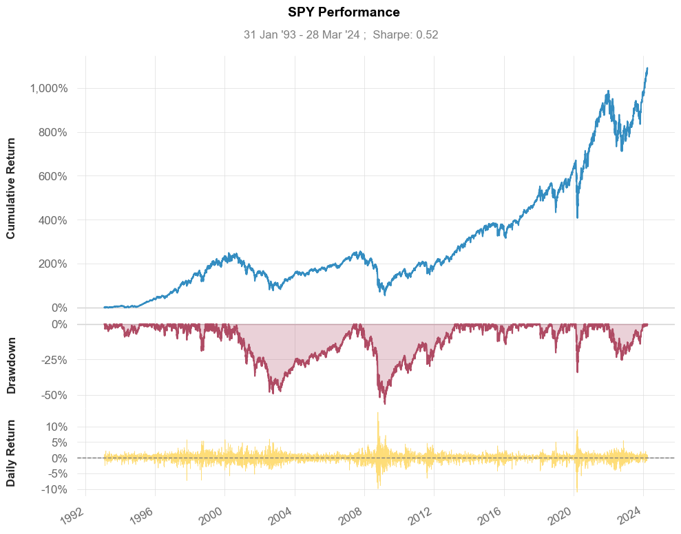
../_images/2874534a9a5bc94c011ed2fd8d507f42aab47c17a57ef049ca4b7aeea5a29c63.png

qs.reports.html(stock, "SPY")

Running the code above will generate a report that looks similar to this:

Link to QuantStats.

6.7.14. kneed: Knee-Point Detection in Time Series#

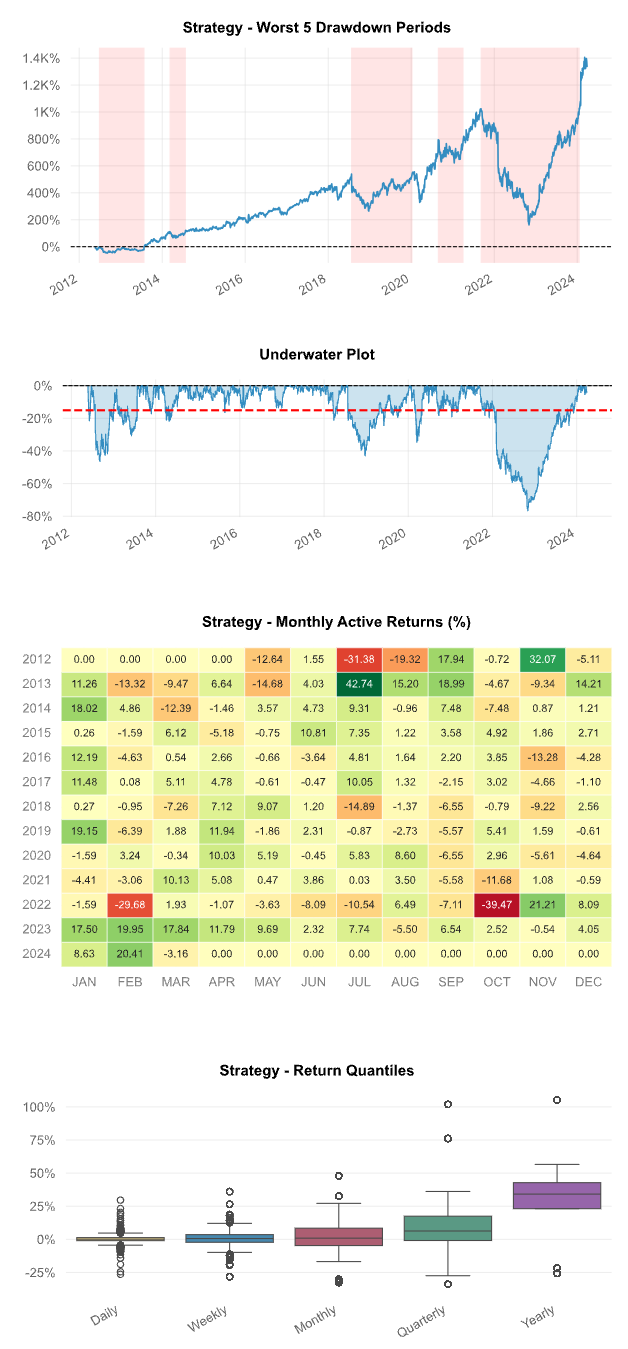
Knee-point detection in time series identifies the point of maximum curvature. The knee point can identify anomalies or outliers in the time series. If a data point is far away from the knee point, it may indicate an anomaly or unexpected behavior.

The kneed library makes it easy to implement knee-point detection in Python.

from kneed import DataGenerator, KneeLocator

x, y = DataGenerator.figure2()

kneedle = KneeLocator(x, y, S=1.0, curve="concave", direction="increasing")
kneedle.plot_knee_normalized()

../_images/5faaf85607e549cde6ceb7ea2c20b7e64fdec801c6ad304f664018113f273e09.png

Link to kneed.

6.7.15. Visualize Time Series with `plot_series`#

Analyzing time series data and forecasts can be challenging without proper visualization. Raw data often lacks context or insights, making it difficult to interpret trends, anomalies, and forecast accuracy effectively.

import matplotlib.pyplot as plt
import numpy as np
import pandas as pd

# Example of a simple time series dataset
np.random.seed(42)
date_range = pd.date_range(start="2023-01-01", periods=30, freq="D")
data = {
    "unique_id": ["id_1"] * 30,
    "ds": date_range,
    "y": np.random.randn(30).cumsum(),  # Simulating cumulative values
}
df = pd.DataFrame(data)

## Plotting without any framework - raw visualization
plt.plot(df["ds"], df["y"], label="Observed Values")
plt.xlabel("Date")
plt.ylabel("Value")
plt.title("Raw Time Series Visualization")
plt.legend()
plt.grid(True)
plt.show()

plot_series from Nixtla’s utilsforecast offers advanced and customizable plotting capabilities for time series data, enabling clear visualization of forecasts, anomalies, and prediction intervals.

Utilize plot_series to visualize time series data and forecasts using the following steps:

6.7.16. Preparing the Data#

generate_series is a utility to simulate time series data, including training and testing datasets. Below, we create a dataset with 4 time series, each containing a trend, and split it into training and testing sets.

from utilsforecast.data import generate_series

## Generate example time series data
level = [80, 95]  # Confidence intervals
series = generate_series(
    n_series=1,  # Number of time series
    freq="D",  # Daily frequency
    equal_ends=True,
    with_trend=True,
    n_models=2,  # Number of forecast models
    level=level,
)

## Split data into training and testing
test_pd = series.groupby("unique_id", observed=True).tail(10).copy()
train_pd = series.drop(test_pd.index)

6.7.17. Visualizing Using `plot_series`#

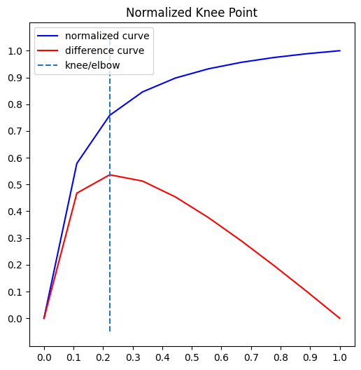
We utilize the plot_series function to visualize both the training and forecasted data for selected time series.

import matplotlib.pyplot as plt
from utilsforecast.plotting import plot_series

## Style for plots
plt.style.use("ggplot")

## Plot using plot_series
fig = plot_series(
    train_pd,  # Training dataset
    forecasts_df=test_pd,  # Forecast dataset
    ids=[0],  # Select specific time series to plot
    plot_random=False,  # Ensure reproducibility
    level=level,  # Add prediction intervals
    max_insample_length=50,  # Limit insample length
    engine="matplotlib",  # Use matplotlib for visualization
    plot_anomalies=True,  # Highlight anomalies
)

fig

../_images/731ae0a3cb2772a8362b5fafbc88486a25c452efdc138e6ecd3b11f060ea1574.png

The generated plot includes:

The actual observed values from the training dataset.
Forecasted values for the testing dataset.
Highlighted anomalies (if any) based on prediction intervals.
Confidence intervals (80% and 95%) for forecasted data.

The output reveals the time series trends, forecasts, and anomalies. Confidence intervals provide clarity on the uncertainty of predictions, while anomalies indicate deviations from expected patterns.

Link to Plotting - Nixtla.

6.7.18. NeuralForecast: Streamline Neural Forecasting with Familiar Sklearn Syntax#

Neural forecasting methods can enhance the accuracy of forecasting, but they are often difficult to use and computationally expensive.

NeuralForecast provides a simple way to use proven accurate and efficient models, using familiar sklearn syntax. The models available in NeuralForecast range from classic networks like RNN to the latest transformers.

from neuralforecast import NeuralForecast
from neuralforecast.models import NBEATS
from neuralforecast.utils import AirPassengersDF

nf = NeuralForecast(models=[NBEATS(input_size=24, h=12, max_steps=100)], freq="M")

nf.fit(df=AirPassengersDF)
nf.predict()

Link to NeuralForecast.

6.7.19. Scaling Time-Series Forecasting with StatsForecast and Spark#

Traditional time series libraries are typically built to run in-memory on single machines, which poses challenges when handling extremely large datasets.

StatsForecast, however, provides seamless compatibility with Spark, allowing users to perform scalable and efficient time-series forecasting on large datasets directly within Spark.

from pyspark.sql import SparkSession

spark = SparkSession.builder.config(
    "spark.executorEnv.NIXTLA_ID_AS_COL", "1"
).getOrCreate()

from statsforecast.core import StatsForecast
from statsforecast.models import AutoETS
from statsforecast.utils import generate_series
from tqdm.autonotebook import tqdm

n_series = 4
horizon = 7

series = generate_series(n_series)

## Convert to Spark
spark_df = spark.createDataFrame(series)
spark_df.show(5)

/Users/khuyentran/.pyenv/versions/3.8.16/lib/python3.8/site-packages/statsforecast/core.py:27: TqdmExperimentalWarning: Using `tqdm.autonotebook.tqdm` in notebook mode. Use `tqdm.tqdm` instead to force console mode (e.g. in jupyter console)
  from tqdm.autonotebook import tqdm
                                                                                

+---------+-------------------+-------------------+
|unique_id|                 ds|                  y|
+---------+-------------------+-------------------+
|        0|2000-01-01 00:00:00|0.30138168803582194|
|        0|2000-01-02 00:00:00| 1.2724415914984484|
|        0|2000-01-03 00:00:00|  2.211827399669452|
|        0|2000-01-04 00:00:00|  3.322947056533328|
|        0|2000-01-05 00:00:00|  4.218793605631347|
+---------+-------------------+-------------------+
only showing top 5 rows

sf = StatsForecast(models=[AutoETS(season_length=7)], freq="D")

## Returns a Spark DataFrame
sf.forecast(df=spark_df, h=horizon, level=[90]).show(5)

Link to StatsForecast.

6.7.20. Beyond Point Estimates: Leverage Prediction Intervals for Robust Forecasting#

Generating a forecast typically produces a single point estimate, which does not reflect the uncertainty associated with the prediction.

To quantify this uncertainty, we need prediction intervals - a range of values the forecast can take with a given probability. MLForecast allows you to train sklearn models to generate both point forecasts and prediction intervals.

To demonstrate this, let’s consider the following example:

import pandas as pd
from utilsforecast.plotting import plot_series

train = pd.read_csv("https://auto-arima-results.s3.amazonaws.com/M4-Hourly.csv")
test = pd.read_csv("https://auto-arima-results.s3.amazonaws.com/M4-Hourly-test.csv")
train.head()

	unique_id	ds	y
0	H1	1	605.0
1	H1	2	586.0
2	H1	3	586.0
3	H1	4	559.0
4	H1	5	511.0

We’ll only use the first series of the dataset.

n_series = 1
uids = train["unique_id"].unique()[:n_series]
train = train.query("unique_id in @uids")
test = test.query("unique_id in @uids")

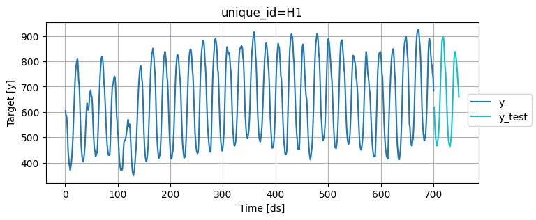
Plot these series using the plot_series function from the utilsforecast library

fig = plot_series(
    df=train,
    forecasts_df=test.rename(columns={"y": "y_test"}),
    models=["y_test"],
    palette="tab10",
)

fig.set_size_inches(8, 3)
fig

../_images/08e1e247888cd50ff3265ddef8d4a0b5752ae26e14b4ec07daa1ab6ff86126ef.png

Train multiple models that follow the sklearn syntax:

from mlforecast import MLForecast
from mlforecast.target_transforms import Differences
from mlforecast.utils import PredictionIntervals
from sklearn.linear_model import LinearRegression
from sklearn.neighbors import KNeighborsRegressor

mlf = MLForecast(
    models=[
        LinearRegression(),
        KNeighborsRegressor(),
    ],
    freq=1,
    target_transforms=[Differences([1])],
    lags=[24 * (i + 1) for i in range(7)],
)

Apply the feature engineering and train the models:

mlf.fit(
    df=train,
    prediction_intervals=PredictionIntervals(n_windows=10, h=48),
)

MLForecast(models=[LinearRegression, KNeighborsRegressor], freq=1, lag_features=['lag24', 'lag48', 'lag72', 'lag96', 'lag120', 'lag144', 'lag168'], date_features=[], num_threads=1)

Generate forecasts with prediction intervals:

## A list of floats with the confidence levels of the prediction intervals
levels = [50, 80, 95]

## Predict the next 48 hours
horizon = 48

## Generate forecasts with prediction intervals
forecasts = mlf.predict(h=horizon, level=levels)
forecasts.head()

	unique_id	ds	LinearRegression	KNeighborsRegressor	LinearRegression-lo-95	LinearRegression-lo-80	LinearRegression-lo-50	LinearRegression-hi-50	LinearRegression-hi-80	LinearRegression-hi-95	KNeighborsRegressor-lo-95	KNeighborsRegressor-lo-80	KNeighborsRegressor-lo-50	KNeighborsRegressor-hi-50	KNeighborsRegressor-hi-80	KNeighborsRegressor-hi-95
0	H1	701	612.454151	615.2	597.550958	601.310692	604.037187	620.871115	623.597610	627.357344	599.090	603.20	609.45	620.95	627.20	631.310
1	H1	702	538.415217	551.6	491.913415	508.094072	527.337321	549.493112	568.736361	584.917018	505.675	534.04	535.85	567.35	569.16	597.525
2	H1	703	496.797892	509.6	458.432874	472.483280	481.705219	511.890565	521.112505	535.162911	475.020	488.28	492.70	526.50	530.92	544.180
3	H1	704	462.689475	474.6	414.114933	435.849278	442.808787	482.570164	489.529672	511.264017	423.700	444.52	451.00	498.20	504.68	525.500
4	H1	705	439.784731	451.6	384.182476	400.101658	419.176045	460.393416	479.467803	495.386986	394.555	411.28	428.15	475.05	491.92	508.645

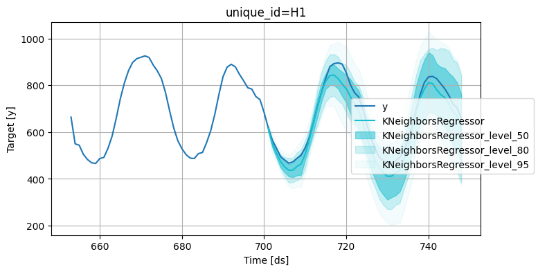
Merge the test data with forecasts:

test_with_forecasts = test.merge(forecasts, how="left", on=["unique_id", "ds"])

Plot the point and the prediction intervals:

levels = [50, 80, 95]
fig = plot_series(
    train,
    test_with_forecasts,
    plot_random=False,
    models=["KNeighborsRegressor"],
    level=levels,
    max_insample_length=48,
    palette="tab10",
)
fig.set_size_inches(8, 4)
fig

../_images/f9dd84ef015aa6a2c31bfde0c69daac1dd76196da6fe0e75d024bce954ad7552.png

Link to MLForecast.

6.7.21. Sliding Window Approach to Time Series Cross-Validation#

Time series cross-validation evaluates a model’s predictive performance by training on past data and testing on subsequent time periods using a sliding window approach.

MLForecast offers an efficient and easy-to-use implementation of this technique.

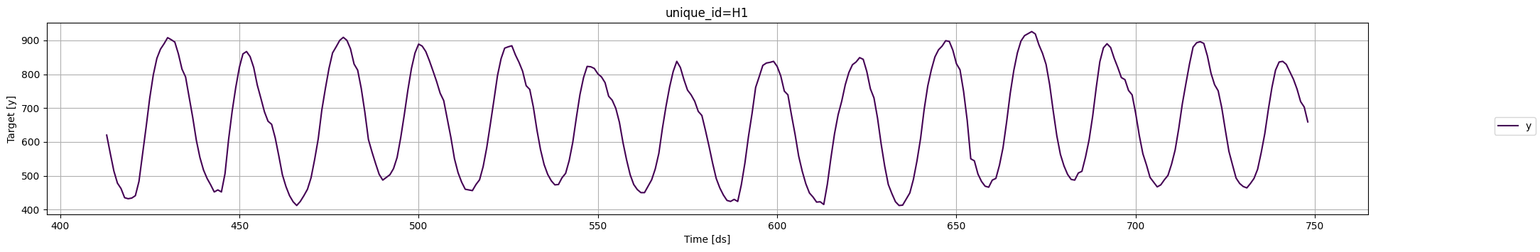
To see how to implement time series cross-validation with MLForecast, let’s start reading a subset of the M4 Competition hourly dataset.

import pandas as pd
from utilsforecast.plotting import plot_series

Y_df = pd.read_csv("https://datasets-nixtla.s3.amazonaws.com/m4-hourly.csv").query(
    "unique_id == 'H1'"
)
print(Y_df)

    unique_id   ds      y
        H1    1  605.0
        H1    2  586.0
        H1    3  586.0
        H1    4  559.0
        H1    5  511.0
..        ...  ...    ...
      H1  744  785.0
      H1  745  756.0
      H1  746  719.0
      H1  747  703.0
      H1  748  659.0

[748 rows x 3 columns]

Plot the time series:

fig = plot_series(Y_df, plot_random=False, max_insample_length=24 * 14)
fig

../_images/d1e74ef1167defcd842de2f93c72a58ea5e62c240ddfc7386a8a67e914e2f749.png

Instantiate a new MLForecast object:

from mlforecast import MLForecast
from mlforecast.target_transforms import Differences
from sklearn.linear_model import LinearRegression

mlf = MLForecast(
    models=[LinearRegression()],
    freq=1,
    target_transforms=[Differences([24])],
    lags=range(1, 25),
)

Once the MLForecast object has been instantiated, we can use the cross_validation method.

For this particular example, we’ll use 3 windows of 24 hours.

# use 3 windows of 24 hours
cross_validation_df = mlf.cross_validation(
    df=Y_df,
    h=24,
    n_windows=3,
)

print(cross_validation_df.head())

  unique_id   ds  cutoff      y  LinearRegression
      H1  677     676  691.0        676.726797
      H1  678     676  618.0        559.559522
      H1  679     676  563.0        549.167938
      H1  680     676  529.0        505.930997
      H1  681     676  504.0        481.981893

We’ll now plot the forecast for each cutoff period.

import matplotlib.pyplot as plt


def plot_cv(df, df_cv, last_n=24 * 14):
    cutoffs = df_cv["cutoff"].unique()
    fig, ax = plt.subplots(
        nrows=len(cutoffs), ncols=1, figsize=(14, 6), gridspec_kw=dict(hspace=0.8)
    )
    for cutoff, axi in zip(cutoffs, ax.flat):
        df.tail(last_n).set_index("ds").plot(ax=axi, y="y")
        df_cv.query("cutoff == @cutoff").set_index("ds").plot(
            ax=axi,
            y="LinearRegression",
            title=f"{cutoff=}",
        )


plot_cv(Y_df, cross_validation_df)

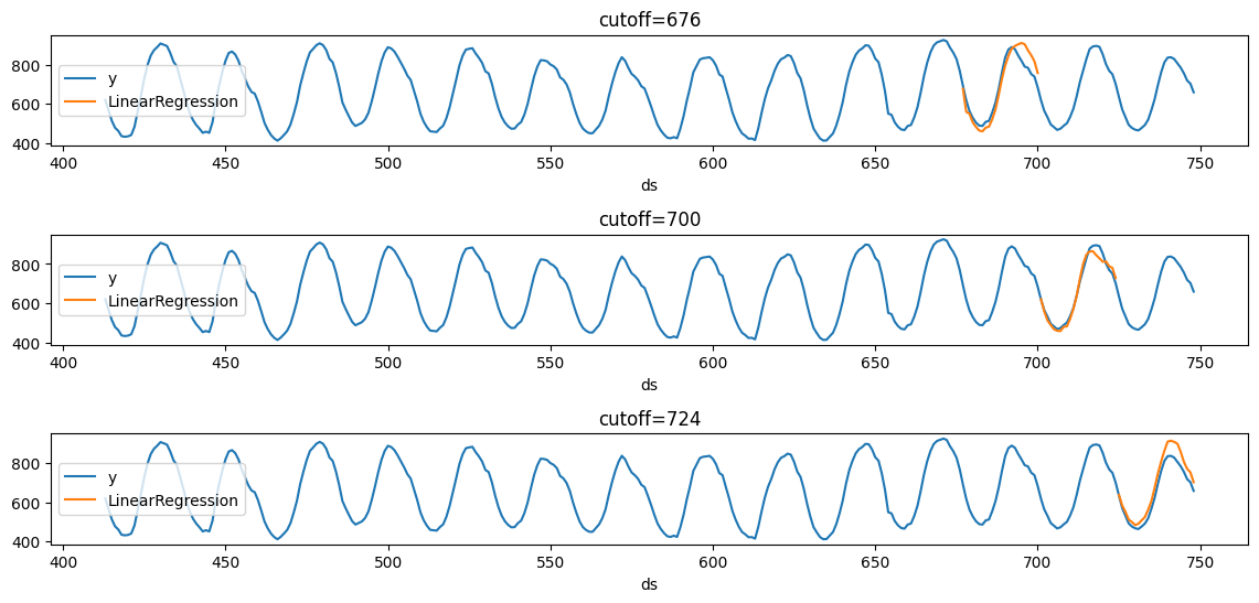
../_images/e7ac75d7a3789e521ef4f5dd5d26dd61a3276e10d56ee7b6c05bea6184ed4791.png

Notice that in each cutoff period, we generated a forecast for the next 24 hours using only the data y before said period.

Link to MLForecast.

6.7.22. Handling Static and Dynamic Features in Time Series Forecasting with MLForecast#

Basic time series data often fails to properly incorporate different types of features.

MLForecast provides a comprehensive solution for handling both static and dynamic features:

import lightgbm as lgb
from mlforecast import MLForecast
from mlforecast.utils import generate_daily_series, generate_prices_for_series

## Generate sample data
series = generate_daily_series(100, equal_ends=True, n_static_features=2)
series = series.rename(columns={"static_0": "store_id", "static_1": "product_id"})

## Generate price catalog (dynamic feature)
prices_catalog = generate_prices_for_series(series)

## Merge static and dynamic features
series_with_prices = series.merge(prices_catalog, how="left")
print(series_with_prices.head(10))

  unique_id         ds           y store_id product_id     price
   id_00 2000-10-05   39.811983       79         45  0.548814
   id_00 2000-10-06  103.274013       79         45  0.715189
   id_00 2000-10-07  176.574744       79         45  0.602763
   id_00 2000-10-08  258.987900       79         45  0.544883
   id_00 2000-10-09  344.940404       79         45  0.423655
   id_00 2000-10-10  413.520305       79         45  0.645894
   id_00 2000-10-11  506.990093       79         45  0.437587
   id_00 2000-10-12   12.688070       79         45  0.891773
   id_00 2000-10-13  111.133819       79         45  0.963663
   id_00 2000-10-14  197.982842       79         45  0.383442

Create and train the forecasting model:

# Create MLForecast model
fcst = MLForecast(
    models=lgb.LGBMRegressor(random_state=0),
    freq="D",
    lags=[7],  # Use 7-day lag
    date_features=["dayofweek"],  # Add day of week as feature
)

## Fit model specifying which features are static
fcst.fit(
    series_with_prices,
    static_features=["store_id", "product_id"],  # Specify static features
)

MLForecast(models=[LGBMRegressor], freq=D, lag_features=['lag7'], date_features=['dayofweek'], num_threads=1)

## Check which features are used for training
print("\nFeatures used for training:")
print(fcst.ts.features_order_)

Features used for training:
['store_id', 'product_id', 'price', 'lag7', 'dayofweek']

Generate predictions:

## Make predictions using future prices
predictions = fcst.predict(
    h=7, X_df=prices_catalog  # Forecast 7 days ahead  # Provide future prices
)
print(predictions.head(10))

  unique_id         ds  LGBMRegressor
   id_00 2001-05-15     421.301684
   id_00 2001-05-16     497.335181
   id_00 2001-05-17      20.108545
   id_00 2001-05-18     101.930145
   id_00 2001-05-19     184.264253
   id_00 2001-05-20     260.803990
   id_00 2001-05-21     343.501305
   id_01 2001-05-15     118.299009
   id_01 2001-05-16     148.793503
   id_01 2001-05-17     184.066779

Link to MLForecast

6.7.23. Hierarchical Forecasting in Python#

In complex datasets, forecasts at detailed levels (e.g., regions, products) should align with higher-level forecasts (e.g., countries, categories). Inconsistent forecasts can lead to poor decisions.

Hierarchical forecasting ensures forecasts are consistent across all levels to reconcile and match forecasts from lower to higher levels.

HierarchicalForecast, an open-source library from Nixtla, offers tools and methods specifically designed for creating and reconciling hierarchical forecasts.

For illustrative purposes, consider a sales dataset with the following columns:

Country: The country where the sales occurred.
Region: The region within the country.
State: The state within the region.
Purpose: The purpose of the sale (e.g., Business, Leisure).
ds: The date of the sale.
y: The sales amount.

import numpy as np
import pandas as pd

%%capture
Y_df = pd.read_csv(
    "https://raw.githubusercontent.com/Nixtla/transfer-learning-time-series/main/datasets/tourism.csv"
)
Y_df = Y_df.rename({"Trips": "y", "Quarter": "ds"}, axis=1)
Y_df.insert(0, "Country", "Australia")
Y_df = Y_df[["Country", "State", "Region", "Purpose", "ds", "y"]]
Y_df["ds"] = Y_df["ds"].str.replace(r"(\d+) (Q\d)", r"\1-\2", regex=True)
Y_df["ds"] = pd.to_datetime(Y_df["ds"])
Y_df.head()

The dataset can be grouped in the following non-strictly hierarchical structure:

Country
Country, State
Country, Purpose
Country, State, Region
Country, State, Purpose
Country, State, Region, Purpose

spec = [
    ["Country"],
    ["Country", "State"],
    ["Country", "Purpose"],
    ["Country", "State", "Region"],
    ["Country", "State", "Purpose"],
    ["Country", "State", "Region", "Purpose"],
]

Using the aggregate function from HierarchicalForecast we can get the full set of time series.

from hierarchicalforecast.utils import aggregate

Y_df, S_df, tags = aggregate(Y_df, spec)
Y_df = Y_df.reset_index()
Y_df.sample(10)

	unique_id	ds	y
12251	Australia/New South Wales/Outback NSW/Business	2000-10-01	23.780860
33131	Australia/Western Australia/Australia's North ...	2000-10-01	45.648865
22034	Australia/South Australia/Fleurieu Peninsula/O...	2006-07-01	0.000000
31119	Australia/Victoria/Phillip Island/Visiting	2017-10-01	58.063034
7671	Australia/New South Wales/Other	2015-10-01	405.891206
18339	Australia/Queensland/Mackay/Business	2002-10-01	54.135284
23043	Australia/South Australia/Limestone Coast/Visi...	1998-10-01	32.604546
22129	Australia/South Australia/Fleurieu Peninsula/V...	2010-04-01	44.738053
11349	Australia/New South Wales/Hunter/Business	2015-04-01	132.226040
16599	Australia/Queensland/Brisbane/Other	2007-10-01	70.490809

Get all the distinct ‘Country/Purpose’ combinations present in the dataset:

tags["Country/Purpose"]

array(['Australia/Business', 'Australia/Holiday', 'Australia/Other',
       'Australia/Visiting'], dtype=object)

We use the final two years (8 quarters) as test set.

Y_test_df = Y_df.groupby("unique_id").tail(8)
Y_train_df = Y_df.drop(Y_test_df.index)

Y_test_df = Y_test_df.set_index("unique_id")
Y_train_df = Y_train_df.set_index("unique_id")

Y_train_df.groupby("unique_id").size()

unique_id
Australia                                                72
Australia/ACT                                            72
Australia/ACT/Business                                   72
Australia/ACT/Canberra                                   72
Australia/ACT/Canberra/Business                          72
                                                         ..
Australia/Western Australia/Experience Perth/Other       72
Australia/Western Australia/Experience Perth/Visiting    72
Australia/Western Australia/Holiday                      72
Australia/Western Australia/Other                        72
Australia/Western Australia/Visiting                     72
Length: 425, dtype: int64

The following cell generates base forecasts for each time series in Y_df using the ETS model. The forecasts and fitted values are stored in Y_hat_df and Y_fitted_df, respectively.

%%capture
from statsforecast.core import StatsForecast
from statsforecast.models import ETS

fcst = StatsForecast(
    df=Y_train_df, models=[ETS(season_length=4, model="ZZA")], freq="QS", n_jobs=-1
)
Y_hat_df = fcst.forecast(h=8, fitted=True)
Y_fitted_df = fcst.forecast_fitted_values()

Since Y_hat_df contains forecasts that are not coherent—meaning forecasts at detailed levels (e.g., by State, Region, Purpose) may not align with those at higher levels (e.g., by Country, State, Purpose)—we will use the HierarchicalReconciliation class with the BottomUp approach to ensure coherence.

from hierarchicalforecast.core import HierarchicalReconciliation
from hierarchicalforecast.methods import BottomUp

reconcilers = [BottomUp()]
hrec = HierarchicalReconciliation(reconcilers=reconcilers)
Y_rec_df = hrec.reconcile(Y_hat_df=Y_hat_df, Y_df=Y_fitted_df, S=S_df, tags=tags)

The dataframe Y_rec_df contains the reconciled forecasts.

Y_rec_df.head()

	ds	ETS	ETS/BottomUp
unique_id
Australia	2016-01-01	25990.068359	24380.257812
Australia	2016-04-01	24458.490234	22902.765625
Australia	2016-07-01	23974.056641	22412.982422
Australia	2016-10-01	24563.455078	23127.439453
Australia	2017-01-01	25990.068359	24516.759766

Link to Hierarchical Forecast

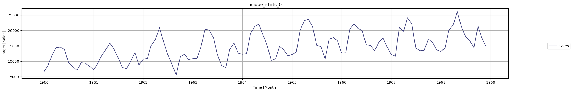
6.7.24. Generative Pre-trained Forecasting with TimeGPT#

TimeGPT is a powerful generative pre-trained forecasting model that can generate accurate forecasts for new time series without the need for training. TimeGPT can be used across a variety of tasks including demand forecasting, anomaly detection, financial forecasting, and more.

from nixtla import NixtlaClient

nixtla_client = NixtlaClient(api_key="my_api_key_provided_by_nixtla")

import pandas as pd

time_column = "Month"
value_column = "Sales"
df = pd.read_csv(
    "https://raw.githubusercontent.com/jbrownlee/Datasets/master/monthly-car-sales.csv",
    parse_dates=[time_column],
)

df.head()

	Month	Sales
0	1960-01-01	6550
1	1960-02-01	8728
2	1960-03-01	12026
3	1960-04-01	14395
4	1960-05-01	14587

nixtla_client.plot(df, time_col=time_column, target_col=value_column)

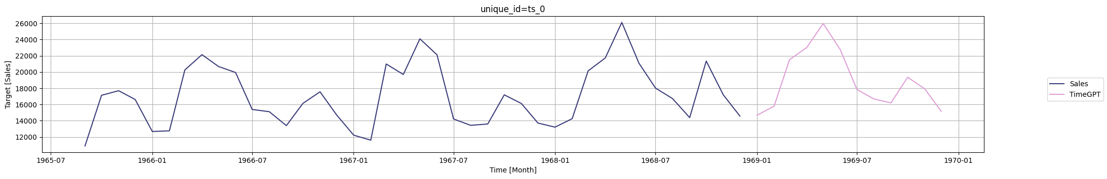
../_images/02af13078cc214a465c7479146e5b3f39f55720c07660db6fd5f271df5187ada.png

timegpt_fcst_df = nixtla_client.forecast(
    df=df, h=12, freq="MS", time_col=time_column, target_col=value_column
)
timegpt_fcst_df.head()

INFO:nixtla.nixtla_client:Validating inputs...
INFO:nixtla.nixtla_client:Preprocessing dataframes...
INFO:nixtla.nixtla_client:Restricting input...
INFO:nixtla.nixtla_client:Calling Forecast Endpoint...

	Month	TimeGPT
0	1969-01-01	14672.101562
1	1969-02-01	15793.253906
2	1969-03-01	21517.191406
3	1969-04-01	22996.332031
4	1969-05-01	25959.019531

nixtla_client.plot(
    df,
    timegpt_fcst_df,
    time_col=time_column,
    target_col=value_column,
    max_insample_length=40,
)

../_images/6ec4c570eb2332f0e21fd89161365ee9af76f6c1be3a04ea87223cf18f5a2515.png

Link to TimeGPT.

6.7.25. Automate Time Series Feature Engineering with tsfresh#

Data scientists spend much of their time cleaning data or building features. While the former is unavoidable, the latter can be automated.

tsfresh uses a robust feature selection algorithm to automatically extract relevant time series features, freeing up data scientists’ time.

To demonstrate this, start with loading an example dataset:

from tsfresh.examples.robot_execution_failures import (
    download_robot_execution_failures,
    load_robot_execution_failures,
)

download_robot_execution_failures()
timeseries, y = load_robot_execution_failures()

timeseries.head()

	id	time	F_x	F_y	F_z	T_x	T_y
0	1	0	-1	-1	63	-3	-1
1	1	1	0	0	62	-3	-1
2	1	2	-1	-1	61	-3	0
3	1	3	-1	-1	63	-2	-1
4	1	4	-1	-1	63	-3	-1

Extract features and select only relevant features for each time series.

from tsfresh import extract_relevant_features

# extract relevant features
features_filtered = extract_relevant_features(
    timeseries, y, column_id="id", column_sort="time"
)

Feature Extraction: 100%|██████████| 20/20 [00:05<00:00,  3.83it/s]

You can now use the features in features_filtered to train your classification model.

# perform model training with the extracted features

Link to tsfresh.

6.7.26. tsmoothie: Fast and Flexible Tool for Exponential Smoothing#

Exponential smoothing is useful for capturing the underlying pattern in the data, especially for data with a strong trend or seasonal component.

tsmoothie is designed to be fast and efficient and provides a wide range of smoothing techniques.

To see how tsmoothie works, let’s generate a single random walk time series of length 200 using the sim_randomwalk() function.

import matplotlib.pyplot as plt
import numpy as np
from tsmoothie.smoother import LowessSmoother
from tsmoothie.utils_func import sim_randomwalk

# generate a random walk of length 200
np.random.seed(123)
data = sim_randomwalk(n_series=1, timesteps=200, process_noise=10, measure_noise=30)

Next, create a LowessSmoother object with a smooth_fraction of 0.1 (i.e., 10% of the data points are used for local regression) and 1 iteration. We then apply the smoothing operation to the data using the smooth() method.

# operate smoothing
smoother = LowessSmoother(smooth_fraction=0.1, iterations=1)
smoother.smooth(data)

<tsmoothie.smoother.LowessSmoother>

After smoothing the data, we use the get_intervals() method of the LowessSmoother object to calculate the lower and upper bounds of the prediction interval for the smoothed time series.

# generate intervals
low, up = smoother.get_intervals("prediction_interval")

Finally, we plot the smoothed time series (as a blue line), and the prediction interval (as a shaded region) using matplotlib.

# plot the smoothed time series with intervals
plt.figure(figsize=(10, 5))

plt.plot(smoother.smooth_data[0], linewidth=3, color="blue")
plt.plot(smoother.data[0], ".k")
plt.title(f"timeseries")
plt.xlabel("time")

plt.fill_between(range(len(smoother.data[0])), low[0], up[0], alpha=0.3)

<matplotlib.collections.PolyCollection at 0x15b25a8e0>

../_images/840e0ccc6c7a2320f574a46fe4268a67c7d9ae598452c43ea0f50d604fc8c185.png

This graph effectively highlights the trend and seasonal components present in the time series data through the use of a smoothed representation.

Link to tsmoothie.

6.7.27. Backtesting: Assess Trading Strategy Performance Effortlessly in Python#

Evaluating trading strategies’ effectiveness is crucial for financial decision-making, but it’s challenging due to the complexities of historical data analysis and strategy testing.

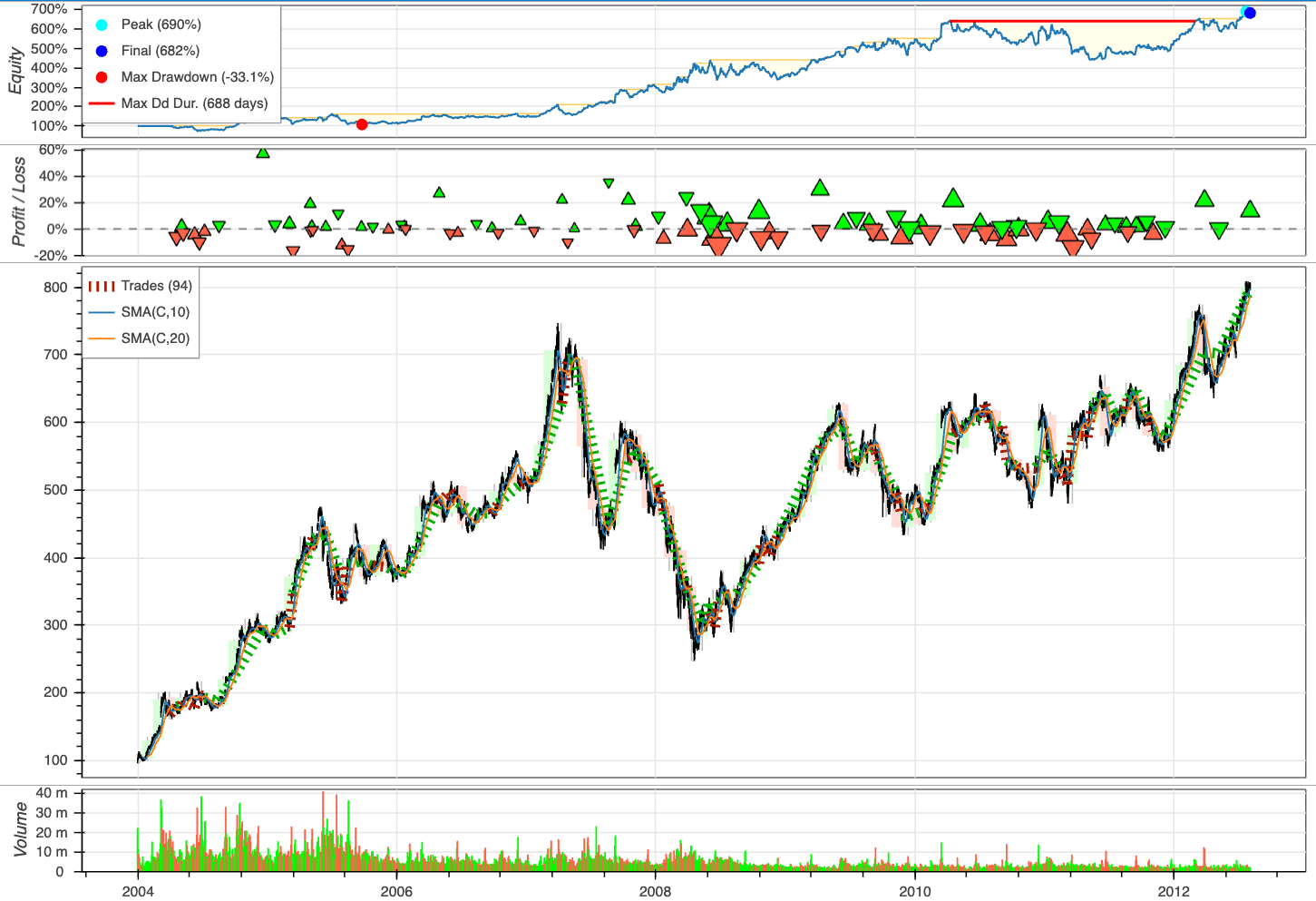
Backtesting allows users to simulate trades based on historical data and visualize the outcomes through interactive plots in three lines of code.

To see how Backtesting works, let’s create our first strategy to backtest on these Google data, a simple moving average (MA) cross-over strategy.

from backtesting.test import GOOG

print(GOOG.tail())

             Open    High     Low   Close   Volume
2013-02-25  802.3  808.41  790.49  790.77  2303900
2013-02-26  795.0  795.95  784.40  790.13  2202500
2013-02-27  794.8  804.75  791.11  799.78  2026100
2013-02-28  801.1  806.99  801.03  801.20  2265800
2013-03-01  797.8  807.14  796.15  806.19  2175400

import pandas as pd


def SMA(values, n):
    """
    Return simple moving average of `values`, at
    each step taking into account `n` previous values.
    """
    return pd.Series(values).rolling(n).mean()

from backtesting import Strategy
from backtesting.lib import crossover


class SmaCross(Strategy):
    # Define the two MA lags as *class variables*
    # for later optimization
    n1 = 10
    n2 = 20

    def init(self):
        # Precompute the two moving averages
        self.sma1 = self.I(SMA, self.data.Close, self.n1)
        self.sma2 = self.I(SMA, self.data.Close, self.n2)

    def next(self):
        # If sma1 crosses above sma2, close any existing
        # short trades, and buy the asset
        if crossover(self.sma1, self.sma2):
            self.position.close()
            self.buy()

        # Else, if sma1 crosses below sma2, close any existing
        # long trades, and sell the asset
        elif crossover(self.sma2, self.sma1):
            self.position.close()
            self.sell()

To assess the performance of our investment strategy, we will instantiate a Backtest object, using Google stock data as our asset of interest and incorporating the SmaCross strategy class. We’ll start with an initial cash balance of 10,000 units and set the broker’s commission to a realistic rate of 0.2%.

from backtesting import Backtest

bt = Backtest(GOOG, SmaCross, cash=10_000, commission=0.002)
stats = bt.run()
stats

Start                     2004-08-19 00:00:00
End                       2013-03-01 00:00:00
Duration                   3116 days 00:00:00
Exposure Time [%]                   97.067039
Equity Final [$]                  68221.96986
Equity Peak [$]                   68991.21986
Return [%]                         582.219699
Buy & Hold Return [%]              703.458242
Return (Ann.) [%]                   25.266427
Volatility (Ann.) [%]               38.383008
Sharpe Ratio                         0.658271
Sortino Ratio                        1.288779
Calmar Ratio                         0.763748
Max. Drawdown [%]                  -33.082172
Avg. Drawdown [%]                   -5.581506
Max. Drawdown Duration      688 days 00:00:00
Avg. Drawdown Duration       41 days 00:00:00
# Trades                                   94
Win Rate [%]                        54.255319
Best Trade [%]                       57.11931
Worst Trade [%]                    -16.629898
Avg. Trade [%]                       2.074326
Max. Trade Duration         121 days 00:00:00
Avg. Trade Duration          33 days 00:00:00
Profit Factor                        2.190805
Expectancy [%]                       2.606294
SQN                                  1.990216
_strategy                            SmaCross
_equity_curve                             ...
_trades                       Size  EntryB...
dtype: object

Plot the outcomes:

bt.plot()

Link to Backtesting.

6.7.28. Chronos: Unleashing Pre-trained Language Models for Time Series Forecasting#

Probabilistic time series forecasting helps data scientists and analysts predict future values with uncertainty estimates. To leverage pre-trained language models for accurate time series predictions, use Chronos.

The power of Chronos lies in its ability to generate accurate forecasts right out of the box, eliminating the need for extensive model training or fine-tuning in many cases.

Here’s a quick example of using Chronos for forecasting:

import pandas as pd
import torch
from chronos import ChronosPipeline

pipeline = ChronosPipeline.from_pretrained(
    "amazon/chronos-t5-small", torch_dtype=torch.bfloat16
)

df = pd.read_csv(
    "https://raw.githubusercontent.com/AileenNielsen/TimeSeriesAnalysisWithPython/master/data/AirPassengers.csv"
)

# forecast shape: [num_series, num_samples, prediction_length]
forecast = pipeline.predict(
    context=torch.tensor(df["#Passengers"]), prediction_length=12, num_samples=20
)

This code loads the air passenger data, uses the pretrained Chronos model to generate 20 possible forecasts for the next 12 months, and then calculates the median forecast along with a 90% prediction interval.

The Chronos model internally transforms the numerical time series into tokens, processes them through a language model architecture, and then converts the output back into numerical forecasts. This approach allows it to capture complex patterns and dependencies in the data, potentially outperforming traditional forecasting methods, especially in zero-shot scenarios where the model hasn’t been specifically trained on the target time series.

Link to Chronos.

	id	time	F_x	F_y	F_z	T_x	T_y
0	1	0	-1	-1	63	-3	-1
1	1	1	0	0	62	-3	-1
2	1	2	-1	-1	61	-3	0
3	1	3	-1	-1	63	-2	-1
4	1	4	-1	-1	63	-3	-1

	id	time	F_x	F_y	F_z	T_x	T_y
0	1	0	-1	-1	63	-3	-1
1	1	1	0	0	62	-3	-1
2	1	2	-1	-1	61	-3	0
3	1	3	-1	-1	63	-2	-1
4	1	4	-1	-1	63	-3	-1