6.11. Better Pandas#
This section cover tools to make your experience with Pandas a litte bit better.
6.11.1. tqdm: Add Progress Bar to Your Pandas Apply#
Show code cell content
!pip install tqdm
If you want to keep informed about the progress of a pandas apply operation, use tqdm.
import time

import pandas as pd
from tqdm import tqdm

df = pd.DataFrame({"a": [1, 2, 3, 4, 5], "b": [2, 3, 4, 5, 6]})

tqdm.pandas()


def func(row):
    time.sleep(1)
    return row + 1


df["a"].progress_apply(func)
100%|████████████████████████████████████████████████████████████████████████████████████████████████████████████████████| 5/5 [00:05<00:00, 1.00s/it]
0    2
1    3
2    4
3    5
4    6
Name: a, dtype: int64
6.11.2. pandarallel: A Simple Tool to Parallelize Pandas Operations#
Show code cell content
!pip install pandarallel
If you want to parallelize your Pandas operations on all available CPUs by adding only one line of code, try pandarallel.
import pandas as pd
from numpy.random import randint
from pandarallel import pandarallel

df = pd.DataFrame(
    {
        "a": randint(0, 100, size=10000),
        "b": randint(0, 100, size=10000),
        "c": randint(0, 100, size=10000),
    }
)

pandarallel.initialize(progress_bar=True)
df.parallel_apply(lambda x: x**2)
INFO: Pandarallel will run on 8 workers.
INFO: Pandarallel will use standard multiprocessing data transfer (pipe) to transfer data between the main process and workers.
| a | b | c | |
|---|---|---|---|
| 0 | 3025 | 324 | 441 |
| 1 | 1 | 6561 | 5329 |
| 2 | 2025 | 4900 | 1024 |
| 3 | 25 | 5776 | 25 |
| 4 | 16 | 8100 | 3364 |
| ... | ... | ... | ... |
| 9995 | 49 | 676 | 4761 |
| 9996 | 3721 | 6889 | 4 |
| 9997 | 4225 | 9025 | 1156 |
| 9998 | 361 | 9 | 529 |
| 9999 | 5041 | 25 | 81 |
10000 rows × 3 columns
6.11.3. PandasAI: Gain Insights From Your pandas DataFrame With AI#
Show code cell content
!pip install pandasai
If you want to quickly gain insights from your pandas DataFrame with AI, use PandasAI. PandasAI serves as:
A tool to analyze your DataFrame
Not a tool to process your DataFrame
import pandas as pd

df = pd.read_csv(
    "https://raw.githubusercontent.com/mwaskom/seaborn-data/master/flights.csv"
)
df.head(10)
| year | month | passengers | |
|---|---|---|---|
| 0 | 1949 | January | 112 |
| 1 | 1949 | February | 118 |
| 2 | 1949 | March | 132 |
| 3 | 1949 | April | 129 |
| 4 | 1949 | May | 121 |
| 5 | 1949 | June | 135 |
| 6 | 1949 | July | 148 |
| 7 | 1949 | August | 148 |
| 8 | 1949 | September | 136 |
| 9 | 1949 | October | 119 |
df.head(5)
| year | month | passengers | |
|---|---|---|---|
| 0 | 1949 | January | 112 |
| 1 | 1949 | February | 118 |
| 2 | 1949 | March | 132 |
| 3 | 1949 | April | 129 |
| 4 | 1949 | May | 121 |
from pandasai import PandasAI
from pandasai.llm.openai import OpenAI

## Instantiate a LLM
llm = OpenAI(api_token="YOUR_API_TOKEN")

## Use pandasai
pandas_ai = PandasAI(llm, conversational=False)
print(
    pandas_ai.run(
        df,
        prompt="Which month of the years has the highest number of passengers on average?",
    )
)
The month with the highest average number of passengers is: July
print(
    pandas_ai.run(
        df, prompt="Which are the five years with the highest passenger numbers?"
    )
)
year
1960    5714
1959    5140
1958    4572
1957    4421
1956    3939
Name: passengers, dtype: int64
print(pandas_ai.run(df, prompt="Within what range of years does the dataset span?"))
        year     month  passengers
0 1949-01-01   January         112
1 1949-01-01  February         118
2 1949-01-01     March         132
3 1949-01-01     April         129
4 1949-01-01       May         121
The dataset spans from 1949 to 1960.
6.11.4. Combine SQL and Python Efficiently with Ibis#
Show code cell content
!pip install 'ibis-framework[duckdb,examples]'
Data scientists often need to leverage SQL for database queries and Python for advanced data manipulation.
Ibis allows seamless integration of SQL and Python, enabling users to interact with databases using SQL while performing complex operations in Python.
To mix SQL and Python using Ibis:
import ibis

## Enable interactive mode
ibis.options.interactive = True

## Load example data
t = ibis.examples.penguins.fetch()

## Perform an SQL query on the Ibis table
a = t.sql("SELECT species, island, count(*) AS count FROM penguins GROUP BY 1, 2")

## Continue with Python operations
b = a.order_by("count")
print(b)
┏━━━━━━━━━━━┳━━━━━━━━━━━┳━━━━━━━┓
┃ species   ┃ island    ┃ count ┃
┡━━━━━━━━━━━╇━━━━━━━━━━━╇━━━━━━━┩
│ string    │ string    │ int64 │
├───────────┼───────────┼───────┤
│ Adelie    │ Biscoe    │    44 │
│ Adelie    │ Torgersen │    52 │
│ Adelie    │ Dream     │    56 │
│ Chinstrap │ Dream     │    68 │
│ Gentoo    │ Biscoe    │   124 │
└───────────┴───────────┴───────┘
Here’s the breakdown:
t.sql(): Enables SQL queries directly on the Ibis table.order_by("count"): Applies Pythonic dataframe operations on the SQL query result.
6.11.5. fugue: Use pandas Functions on the Spark and Dask Engines.#
Show code cell content
!pip install fugue pyspark
Wouldn’t it be nice if you can leverage Spark or Dask to parallelize data science workloads using pandas syntax? Fugue allows you to do exactly that.
Fugue provides the transform function allowing users to use pandas functions on the Spark and Dask engines.
from typing import Dict

import pandas as pd
from fugue import transform
from fugue_spark import SparkExecutionEngine

input_df = pd.DataFrame({"id": [0, 1, 2], "fruit": (["apple", "banana", "orange"])})
map_price = {"apple": 2, "banana": 1, "orange": 3}


def map_price_to_fruit(df: pd.DataFrame, mapping: dict) -> pd.DataFrame:
    df["price"] = df["fruit"].map(mapping)
    return df


df = transform(
    input_df,
    map_price_to_fruit,
    schema="*, price:int",
    params=dict(mapping=map_price),
    engine=SparkExecutionEngine,
)
df.show()
21/10/01 11:17:05 WARN Utils: Your hostname, khuyen-Precision-7740 resolves to a loopback address: 127.0.1.1; using 192.168.1.90 instead (on interface wlp111s0)
21/10/01 11:17:05 WARN Utils: Set SPARK_LOCAL_IP if you need to bind to another address
WARNING: An illegal reflective access operation has occurred
WARNING: Illegal reflective access by org.apache.spark.unsafe.Platform (file:/home/khuyen/book/venv/lib/python3.8/site-packages/pyspark/jars/spark-unsafe_2.12-3.1.2.jar) to constructor java.nio.DirectByteBuffer(long,int)
WARNING: Please consider reporting this to the maintainers of org.apache.spark.unsafe.Platform
WARNING: Use --illegal-access=warn to enable warnings of further illegal reflective access operations
WARNING: All illegal access operations will be denied in a future release
21/10/01 11:17:05 WARN NativeCodeLoader: Unable to load native-hadoop library for your platform... using builtin-java classes where applicable
Using Spark's default log4j profile: org/apache/spark/log4j-defaults.properties
Setting default log level to "WARN".
To adjust logging level use sc.setLogLevel(newLevel). For SparkR, use setLogLevel(newLevel).
21/10/01 11:17:06 WARN Utils: Service 'SparkUI' could not bind on port 4040. Attempting port 4041.
[Stage 2:===============>                                          (3 + 8) / 11]
+---+------+-----+
| id| fruit|price|
+---+------+-----+
|  0| apple|    2|
|  1|banana|    1|
|  2|orange|    3|
+---+------+-----+
[Stage 2:==========================================> (8 + 3) / 11]
6.11.6. Simplifying Geographic Calculations with GeoPandas#
Show code cell content
!pip install geopandas
Working with geographic data in Python without proper tools can be complex and cumbersome.
Example of working with geographic data without specialized tools:
## Manually handling coordinates and spatial operations
import numpy as np
import pandas as pd

## Complex manual handling of polygon coordinates
df = pd.DataFrame(
    {
        "name": ["Area1", "Area2"],
        "coordinates": [[(0, 0), (1, 0), (1, 1)], [(2, 0), (3, 0), (3, 1), (2, 1)]],
    }
)


## Calculate area
def calculate_polygon_area(coordinates):
    x_coords = [point[0] for point in coordinates]
    y_coords = [point[1] for point in coordinates]

    # Add first point to end to close the polygon
    x_shifted = x_coords[1:] + x_coords[:1]
    y_shifted = y_coords[1:] + y_coords[:1]

    # Calculate using shoelace formula
    first_sum = sum(x * y for x, y in zip(x_coords, y_shifted))
    second_sum = sum(x * y for x, y in zip(x_shifted, y_coords))
    area = 0.5 * abs(first_sum - second_sum)

    return area


df["area"] = df["coordinates"].apply(calculate_polygon_area)
df["area"]
0    0.5
1    1.0
Name: area, dtype: float64
## Calculate parameter
def calculate_perimeter(coordinates):
    # Add first point to end to close the polygon if not already closed
    if coordinates[0] != coordinates[-1]:
        coordinates = coordinates + [coordinates[0]]

    # Calculate distance between consecutive points
    distances = []
    for i in range(len(coordinates) - 1):
        point1 = coordinates[i]
        point2 = coordinates[i + 1]
        # Euclidean distance formula
        distance = np.sqrt((point2[0] - point1[0]) ** 2 + (point2[1] - point1[1]) ** 2)
        distances.append(distance)

    return sum(distances)


df["perimeter"] = df["coordinates"].apply(calculate_perimeter)
df["perimeter"]
0    3.414214
1    4.000000
Name: perimeter, dtype: float64
With GeoPandas, you can:
Work with geometric objects (points, lines, polygons) directly in DataFrame-like structures
Perform spatial operations (intersections, unions, buffers) easily
Visualize geographic data with simple plotting commands
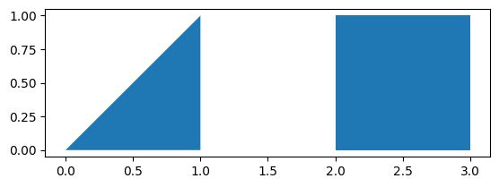
Example using GeoPandas:
import geopandas
from shapely.geometry import Polygon

# Create two polygons
p1 = Polygon([(0, 0), (1, 0), (1, 1)])
p2 = Polygon([(2, 0), (3, 0), (3, 1), (2, 1)])

# Create a GeoSeries from the polygons
g = geopandas.GeoSeries([p1, p2])

## Print the GeoSeries
g
0         POLYGON ((0 0, 1 0, 1 1, 0 0))
1    POLYGON ((2 0, 3 0, 3 1, 2 1, 2 0))
dtype: geometry
## Calculate area
g.area
0    0.5
1    1.0
dtype: float64
## Perimater of each polygon
g.length
0    3.414214
1    4.000000
dtype: float64
import matplotlib.pyplot as plt

g.plot()
plt.show()