Feature Engineer

6.2. Feature Engineer#

This section covers some libraries for feature engineering.

6.2.1. Split Data in a Stratified Fashion in scikit-learn#

Normally, after using scikit-learn’s train_test_split, the proportion of values in the sample will be different from the proportion of values in the entire dataset.

from sklearn.datasets import load_iris
from sklearn.model_selection import train_test_split
import numpy as np

X, y = load_iris(return_X_y=True)
np.bincount(y)

array([50, 50, 50])

X_train, X_test, y_train, y_test = train_test_split(X, y, random_state=0)

# Get count of each class in the train set

np.bincount(y_train)

array([37, 34, 41])

# Get count of each class in the test set

np.bincount(y_test)

array([13, 16,  9])

If you want to keep the proportion of classes in the sample the same as the proportion of classes in the entire dataset, add stratify=y.

X_train, X_test, y_train, y_test = train_test_split(X, y, random_state=0, stratify=y)

np.bincount(y_train)

array([37, 37, 38])

np.bincount(y_test)

array([13, 13, 12])

6.2.2. Strategy to Prevent Data Leakage in Time-correlated Datasets#

If you randomly split time-correlated datasets for machine learning models, your training set may contain future transactions, leading to biased predictions.

To avoid data leakage in time-correlated datasets, split the data by time.

import pandas as pd
from datetime import datetime 

# Create the example dataset
data = {'customer_id': [1, 2, 3, 4, 5],
        'amount': [10.00, 20.00, 15.00, 25.00, 30.00],
        'date': ['2021-01-01', '2021-01-02', '2021-01-03', '2021-01-04', '2021-01-05']}
df = pd.DataFrame(data)

# Convert the date column to datetime format
df['date'] = pd.to_datetime(df['date'])

from sklearn.model_selection import train_test_split

# Split the data randomly into training and test sets
train_data, test_data = train_test_split(df, test_size=0.3, random_state=42)

print(f'Train data:\n{train_data}')
print(f'Test data:\n{test_data}')

Train data:
   customer_id  amount       date
2            3    15.0 2021-01-03
0            1    10.0 2021-01-01
3            4    25.0 2021-01-04
Test data:
   customer_id  amount       date
1            2    20.0 2021-01-02
4            5    30.0 2021-01-05

# Set the cutoff date
cutoff_date = datetime(2021, 1, 4)

# Split the data into training and test sets by time
train_data = df[df['date'] < cutoff_date]
test_data = df[df['date'] >= cutoff_date]

print(f'Train data:\n{train_data}')
print(f'Test data:\n{test_data}')

Train data:
   customer_id  amount       date
0            1    10.0 2021-01-01
1            2    20.0 2021-01-02
2            3    15.0 2021-01-03
Test data:
   customer_id  amount       date
3            4    25.0 2021-01-04
4            5    30.0 2021-01-05

6.2.3. Enhancing Data Handling with scikit-learn’s DataFrame Support#

By default, scikit-learn transformers return a NumPy array. This can pose a challenge if you require the data in a pandas DataFrame for subsequent data processing steps.

Luckily, as of scikit-learn version 1.3.2, you can use the set_output method to obtain the results as a pandas DataFrame.

from sklearn.preprocessing import StandardScaler
from sklearn.impute import SimpleImputer
from sklearn.pipeline import Pipeline
import pandas as pd

# Create a small pandas DataFrame
data = {
    "age": [25, 30, None, 35],
    "income": [50000, 60000, 70000, None],
}
df = pd.DataFrame(data)

scaler = StandardScaler()
scaler.fit_transform(df)

array([[-1.22474487, -1.22474487],
       [ 0.        ,  0.        ],
       [        nan,  1.22474487],
       [ 1.22474487,         nan]])

scaler = StandardScaler().set_output(transform='pandas')
print(scaler.fit_transform(df))

        age    income
-1.224745 -1.224745
0.000000  0.000000
     NaN  1.224745
1.224745       NaN

This method is not limited to individual transformers but can also be applied within a scikit-learn pipeline.

# Create a pipeline with two transformers
pipeline = Pipeline(
    [("imputer", SimpleImputer(strategy="mean")), ("scaler", StandardScaler())]
).set_output(transform="pandas")

# Fit and transform the DataFrame using the pipeline
print(pipeline.fit_transform(df))

        age    income
-1.414214 -1.414214
0.000000  0.000000
0.000000  1.414214
1.414214  0.000000

6.2.4. Efficient Feature Transformation with make_column_transformer in scikit-learn#

The make_column_transformer method in scikit-learn applies different transformations to specific subsets of features in your dataset. This eliminates the need to manually divide and merge data for different transformations.

Additionally, make_column_transformer seamlessly integrates with scikit-learn pipeline, allowing you to combine multiple preprocessing steps and machine learning models into a single pipeline.

import pandas as pd
import numpy as np

data = {
    "cat1": ["A", "B", "A", np.nan, "C"],
    "cat2": ["X", "Y", np.nan, "X", "Z"],
    "num1": [10, np.nan, 15, 25, 30],
    "num2": [1.5, 2.0, np.nan, 2.2, 1.9],
}

X = pd.DataFrame(data)
y = pd.Series([0, 1, 0, 0, 1])

from sklearn.compose import make_column_transformer
from sklearn.pipeline import make_pipeline
from sklearn.preprocessing import StandardScaler, OneHotEncoder
from sklearn.impute import SimpleImputer
from sklearn.linear_model import LogisticRegression


# Define the numeric and categorical features
numeric_features = ["num1", "num2"]
categorical_features = ["cat1", "cat2"]

# Define the transformers and their corresponding columns
numeric_transformer = make_pipeline(SimpleImputer(strategy="median"), StandardScaler())

categorical_transformer = make_pipeline(
    SimpleImputer(strategy="most_frequent"), OneHotEncoder(sparse_output=False)
)
# Create the ColumnTransformer
preprocessor = make_column_transformer(
    (numeric_transformer, numeric_features),
    (categorical_transformer, categorical_features),
    verbose_feature_names_out=False,
).set_output(transform="pandas")

# Fit and transform the data
X_transformed = preprocessor.fit_transform(X)
X_transformed

	num1	num2	cat1_A	cat1_B	cat1_C	cat2_X	cat2_Y	cat2_Z
0	-1.414214	-1.791093	1.0	0.0	0.0	1.0	0.0	0.0
1	0.000000	0.393167	0.0	1.0	0.0	0.0	1.0	0.0
2	-0.707107	0.174741	1.0	0.0	0.0	1.0	0.0	0.0
3	0.707107	1.266871	1.0	0.0	0.0	1.0	0.0	0.0
4	1.414214	-0.043685	0.0	0.0	1.0	0.0	0.0	1.0

pipe = make_pipeline(preprocessor, LogisticRegression())
pipe.fit(X, y)
pipe.predict(X)

array([0, 1, 0, 0, 1])

6.2.5. FunctionTransformer: Build Robust Preprocessing Pipelines with Custom Transformations#

If you want to constructs a transformer from an arbitrary callable, use FunctionTransformer in scikit-learn.

import numpy as np
from sklearn.preprocessing import FunctionTransformer

transformer = FunctionTransformer(np.log1p)
X = np.array([[0, 1], [2, 3]])
transformer.transform(X)

array([[0.        , 0.69314718],
       [1.09861229, 1.38629436]])

The FunctionTransformer enables integrating your custom function seamlessly into scikit-learn’s pipeline framework, making it easier to build complex preprocessing workflows and ensure consistent application of transformations across different datasets.

import pandas as pd
from sklearn.pipeline import Pipeline
from sklearn.linear_model import LogisticRegression
from sklearn.preprocessing import FunctionTransformer
import numpy as np

# Create a simple pandas DataFrame
data = {
    "feature1": [1, 2, 3, 4, 5],
    "feature2": [6, 7, 8, 9, 10],
    "target": [0, 0, 1, 1, 1],
}
df = pd.DataFrame(data)

# Split the DataFrame into features and target
X = df[["feature1", "feature2"]]
y = df["target"]

# Define the FunctionTransformer
log_transformer = FunctionTransformer(np.log1p)


# Define the pipeline
pipeline = Pipeline(
    [("log_transform", log_transformer), ("classifier", LogisticRegression())]
)

# Fit the pipeline on the data
pipeline.fit(X, y)

# Make predictions on new data
new_data = {"feature1": [6, 7], "feature2": [11, 12]}
new_df = pd.DataFrame(new_data)
predictions = pipeline.predict(new_df)

# Print the predictions
print("Predictions:", predictions)

Predictions: [1 1]

6.2.6. Drop Correlated Features#

If you want to remove the correlated variables from a dataframe, use feature_engine.DropCorrelatedFeatures.

import pandas as pd
from sklearn.datasets import make_classification
from feature_engine.selection import DropCorrelatedFeatures

# make dataframe with some correlated variables
X, y = make_classification(
        n_samples=1000,
        n_features=6,
        n_redundant=3,
        n_clusters_per_class=1,
        class_sep=2,
        random_state=0,
    )

# trabsform arrays into pandas df and series
colnames = ["var_" + str(i) for i in range(6)]
X = pd.DataFrame(X, columns=colnames)

X.columns

Index(['var_0', 'var_1', 'var_2', 'var_3', 'var_4', 'var_5'], dtype='object')

X[["var_0", "var_1", "var_2"]].corr()

	var_0	var_1	var_2
var_0	1.000000	0.938936	0.874845
var_1	0.938936	1.000000	0.654745
var_2	0.874845	0.654745	1.000000

Drop the variables with a correlation above 0.8.

tr = DropCorrelatedFeatures(variables=None, method="pearson", threshold=0.8)

Xt = tr.fit_transform(X)

tr.correlated_feature_sets_

[{'var_0', 'var_1', 'var_2'}]

Xt.columns

Index(['var_0', 'var_3', 'var_4', 'var_5'], dtype='object')

Link to feature-engine.

6.2.7. Encode Rare Labels with Feature-engine#

When dealing with features with high cardinality, you might want to mark the rare categories as “Other”. Feature-engine’s RareLabelEncoder makes it easy for you to do so.

from sklearn.datasets import fetch_openml
from feature_engine.encoding import RareLabelEncoder

data = fetch_openml('dating_profile')['data']
data.head(10)

	body_type	diet	drinks	drugs	education	essay0	essay1	essay2	essay3	essay4	...	location	offspring	orientation	pets	religion	sex	sign	smokes	speaks	status
0	a little extra	strictly anything	socially	never	working on college/university	about me:<br />\n<br />\ni would love to think...	currently working as an international agent fo...	making people laugh.<br />\nranting about a go...	the way i look. i am a six foot half asian, ha...	books:<br />\nabsurdistan, the republic, of mi...	...	south san francisco, california	doesn’t have kids, but might want them	straight	likes dogs and likes cats	agnosticism and very serious about it	m	gemini	sometimes	english	single
1	average	mostly other	often	sometimes	working on space camp	i am a chef: this is what that means.<br />\n1...	dedicating everyday to being an unbelievable b...	being silly. having ridiculous amonts of fun w...	None	i am die hard christopher moore fan. i don't r...	...	oakland, california	doesn’t have kids, but might want them	straight	likes dogs and likes cats	agnosticism but not too serious about it	m	cancer	no	english (fluently), spanish (poorly), french (...	single
2	thin	anything	socially	None	graduated from masters program	i'm not ashamed of much, but writing public te...	i make nerdy software for musicians, artists, ...	improvising in different contexts. alternating...	my large jaw and large glasses are the physica...	okay this is where the cultural matrix gets so...	...	san francisco, california	None	straight	has cats	None	m	pisces but it doesn’t matter	no	english, french, c++	available
3	thin	vegetarian	socially	None	working on college/university	i work in a library and go to school. . .	reading things written by old dead people	playing synthesizers and organizing books acco...	socially awkward but i do my best	bataille, celine, beckett. . .<br />\nlynch, j...	...	berkeley, california	doesn’t want kids	straight	likes cats	None	m	pisces	no	english, german (poorly)	single
4	athletic	None	socially	never	graduated from college/university	hey how's it going? currently vague on the pro...	work work work work + play	creating imagery to look at:<br />\nhttp://bag...	i smile a lot and my inquisitive nature	music: bands, rappers, musicians<br />\nat the...	...	san francisco, california	None	straight	likes dogs and likes cats	None	m	aquarius	no	english	single
5	average	mostly anything	socially	None	graduated from college/university	i'm an australian living in san francisco, but...	building awesome stuff. figuring out what's im...	imagining random shit. laughing at aforementio...	i have a big smile. i also get asked if i'm we...	books: to kill a mockingbird, lord of the ring...	...	san francisco, california	doesn’t have kids, but might want them	straight	likes cats	atheism	m	taurus	no	english (fluently), chinese (okay)	single
6	fit	strictly anything	socially	never	graduated from college/university	life is about the little things. i love to lau...	digging up buried treasure	frolicking<br />\nwitty banter<br />\nusing my...	i am the last unicorn	i like books. ones with pictures. reading them...	...	san francisco, california	None	straight	likes dogs and likes cats	None	f	virgo	None	english	single
7	average	mostly anything	socially	never	graduated from college/university	None	writing. meeting new people, spending time wit...	remembering people's birthdays, sending cards,...	i'm rather approachable (a byproduct of being ...	i like: alphabetized lists, aquariums, autobio...	...	san francisco, california	doesn’t have kids, but wants them	straight	likes dogs and likes cats	christianity	f	sagittarius	no	english, spanish (okay)	single
8	None	strictly anything	socially	None	graduated from college/university	None	oh goodness. at the moment i have 4 jobs, so i...	None	i'm freakishly blonde and have the same name a...	i am always willing to try new foods and am no...	...	belvedere tiburon, california	doesn’t have kids	straight	likes dogs and likes cats	christianity but not too serious about it	f	gemini but it doesn’t matter	when drinking	english	single
9	athletic	mostly anything	not at all	never	working on two-year college	my names jake.<br />\ni'm a creative guy and i...	i have an apartment. i like to explore and che...	i'm good at finding creative solutions to prob...	i'm short	i like some tv. i love summer heights high and...	...	san mateo, california	None	straight	likes dogs and likes cats	atheism and laughing about it	m	cancer but it doesn’t matter	no	english (fluently)	single

10 rows × 30 columns

processed = data.dropna(subset=['education'])

In the code below,

tol species the minimum frequency below which a category is considered rare.
replace_with species the value to be used to replace rare categories.
variables specify the list of categorical variables that will be encoded.

encoder = RareLabelEncoder(tol=0.05, variables=["education"], replace_with="Other")
encoded = encoder.fit_transform(processed)

Now the rare categories in the column education are replaced with “Other”.

encoded['education'].sample(10)

                              Other
     graduated from masters program
  graduated from college/university
      working on college/university
                              Other
     graduated from masters program
                              Other
     graduated from masters program
  graduated from college/university
  graduated from college/university
Name: education, dtype: object

Link to feature-engine.

6.2.8. Encode Categorical Data Using Frequency#

Sometimes, count or frequency can be useful features for your model. If you want to replace categories by either the count or the percentage of observations per category, use feature_engine’s CountFrequencyEncoder.

import seaborn as sns
from feature_engine.encoding import CountFrequencyEncoder
from sklearn.model_selection import train_test_split

data = sns.load_dataset("diamonds")

X_train, X_test, y_train, y_test = train_test_split(data, data["price"], random_state=0)
X_train

	carat	cut	color	clarity	depth	table	price	x	y	z
441	0.89	Premium	H	SI2	60.2	59.0	2815	6.26	6.23	3.76
50332	0.70	Very Good	D	SI1	64.0	53.0	2242	5.57	5.61	3.58
35652	0.31	Ideal	G	VVS2	62.7	57.0	907	4.33	4.31	2.71
9439	0.90	Very Good	H	VS1	62.3	59.0	4592	6.12	6.17	3.83
15824	1.01	Good	F	VS2	60.6	62.0	6332	6.52	6.49	3.94
...	...	...	...	...	...	...	...	...	...	...
45891	0.52	Premium	F	VS2	60.7	59.0	1720	5.18	5.14	3.13
52416	0.70	Good	D	SI1	63.6	60.0	2512	5.59	5.51	3.51
42613	0.32	Premium	I	VS1	61.3	58.0	505	4.35	4.39	2.68
43567	0.41	Ideal	G	IF	61.0	57.0	1431	4.81	4.79	2.93
2732	0.91	Ideal	F	SI2	61.1	55.0	3246	6.24	6.19	3.80

40455 rows × 10 columns

In the code below, I encode color and clarity.

# initiate an encoder
encoder = CountFrequencyEncoder(
    encoding_method="frequency", variables=["color", "clarity"]
)

# fit the encoder
encoder.fit(X_train)

# process the data
p_train = encoder.transform(X_train)
p_test = encoder.transform(X_test)

p_test

	carat	cut	color	clarity	depth	table	price	x	y	z
10176	1.10	Ideal	0.152762	0.170436	62.0	55.0	4733	6.61	6.65	4.11
16083	1.29	Ideal	0.152762	0.242022	62.6	56.0	6424	6.96	6.93	4.35
13420	1.20	Premium	0.100531	0.242022	61.1	58.0	5510	6.88	6.80	4.18
20407	1.50	Ideal	0.179409	0.242022	60.9	56.0	8770	7.43	7.36	4.50
8909	0.90	Very Good	0.179409	0.227314	61.7	57.0	4493	6.17	6.21	3.82
...	...	...	...	...	...	...	...	...	...	...
52283	0.59	Very Good	0.182005	0.094401	61.7	59.0	2494	5.37	5.36	3.31
10789	1.00	Fair	0.152762	0.227314	64.8	62.0	4861	6.22	6.13	4.00
1190	0.70	Very Good	0.179409	0.094401	63.2	58.0	2932	5.66	5.60	3.56
3583	0.59	Ideal	0.182005	0.067384	60.7	57.0	3422	5.41	5.45	3.29
40845	0.46	Premium	0.182005	0.227314	61.5	60.0	1173	4.95	4.91	3.03

13485 rows × 10 columns

Link to feature-engine.

6.2.9. Return a DataFrame When Using a scikit-learn’s Transformer#

Applying a scikit-learn’s transformer on your DataFrame will return a NumPy array.

import pandas as pd 
from sklearn.preprocessing import StandardScaler
from feature_engine.wrappers import SklearnTransformerWrapper

df = pd.DataFrame({'a': [1, 2, 3], 'b': [4, 5, 6]})
StandardScaler().fit_transform(df)

array([[-1.22474487, -1.22474487],
       [ 0.        ,  0.        ],
       [ 1.22474487,  1.22474487]])

If you want to return a pandas DataFrame instead, use feature-engine’s SklearnTransformerWrapper along with your scikit-learn’s tranformer.

scaler = SklearnTransformerWrapper(transformer=StandardScaler())
scaler.fit_transform(df)

	a	b
0	-1.224745	-1.224745
1	0.000000	0.000000
2	1.224745	1.224745

Link to feature-engine.

6.2.10. Similarity Encoding for Dirty Categories Using dirty_cat#

To capture the similarities among dirty categories when encoding categorical variables, use dirty_cat’s SimilarityEncoder .

To understand how SimilarityEncoder works, let’s start with the employee_salaries dataset.

from dirty_cat.datasets import fetch_employee_salaries
from dirty_cat import SimilarityEncoder

X = fetch_employee_salaries().X
X.head(10)

	gender	department	department_name	division	assignment_category	employee_position_title	underfilled_job_title	date_first_hired	year_first_hired
0	F	POL	Department of Police	MSB Information Mgmt and Tech Division Records...	Fulltime-Regular	Office Services Coordinator	NaN	09/22/1986	1986
1	M	POL	Department of Police	ISB Major Crimes Division Fugitive Section	Fulltime-Regular	Master Police Officer	NaN	09/12/1988	1988
2	F	HHS	Department of Health and Human Services	Adult Protective and Case Management Services	Fulltime-Regular	Social Worker IV	NaN	11/19/1989	1989
3	M	COR	Correction and Rehabilitation	PRRS Facility and Security	Fulltime-Regular	Resident Supervisor II	NaN	05/05/2014	2014
4	M	HCA	Department of Housing and Community Affairs	Affordable Housing Programs	Fulltime-Regular	Planning Specialist III	NaN	03/05/2007	2007
5	M	POL	Department of Police	PSB 6th District Special Assignment Team	Fulltime-Regular	Police Officer III	NaN	07/16/2007	2007
6	F	FRS	Fire and Rescue Services	EMS Billing	Fulltime-Regular	Accountant/Auditor II	NaN	06/27/2016	2016
7	M	HHS	Department of Health and Human Services	Head Start	Fulltime-Regular	Administrative Specialist II	NaN	11/17/2014	2014
8	M	FRS	Fire and Rescue Services	Recruit Training	Fulltime-Regular	Firefighter/Rescuer III	Firefighter/Rescuer I (Recruit)	12/12/2016	2016
9	F	POL	Department of Police	FSB Traffic Division Automated Traffic Enforce...	Fulltime-Regular	Police Aide	NaN	02/05/2007	2007

dirty_column = "employee_position_title"
X_dirty = df[dirty_column].values
X_dirty[:7]

array(['Office Services Coordinator', 'Master Police Officer',
       'Social Worker IV', 'Resident Supervisor II',
       'Planning Specialist III', 'Police Officer III',
       'Accountant/Auditor II'], dtype=object)

We can see that titles such as ‘Master Police Officer’ and ‘Police Officer III’ are similar. We can use SimilaryEncoder to encode these categories while capturing their similarities.

enc = SimilarityEncoder(similarity="ngram")
X_enc = enc.fit_transform(X_dirty[:10].reshape(-1, 1))
X_enc

array([[0.05882353, 0.03125   , 0.02739726, 0.19008264, 1.        ,
        0.01351351, 0.05555556, 0.20535714, 0.08088235, 0.032     ],
       [0.008     , 0.02083333, 0.056     , 1.        , 0.19008264,
        0.02325581, 0.23076923, 0.56      , 0.01574803, 0.02777778],
       [0.03738318, 0.07317073, 0.05405405, 0.02777778, 0.032     ,
        0.0733945 , 0.        , 0.0625    , 0.06542056, 1.        ],
       [0.11206897, 0.07142857, 0.09756098, 0.01574803, 0.08088235,
        0.07142857, 0.03125   , 0.08108108, 1.        , 0.06542056],
       [0.04761905, 0.3539823 , 0.06976744, 0.02325581, 0.01351351,
        1.        , 0.02      , 0.09821429, 0.07142857, 0.0733945 ],
       [0.0733945 , 0.05343511, 0.14953271, 0.56      , 0.20535714,
        0.09821429, 0.26086957, 1.        , 0.08108108, 0.0625    ],
       [1.        , 0.05      , 0.06451613, 0.008     , 0.05882353,
        0.04761905, 0.01052632, 0.0733945 , 0.11206897, 0.03738318],
       [0.05      , 1.        , 0.03378378, 0.02083333, 0.03125   ,
        0.3539823 , 0.02631579, 0.05343511, 0.07142857, 0.07317073],
       [0.06451613, 0.03378378, 1.        , 0.056     , 0.02739726,
        0.06976744, 0.        , 0.14953271, 0.09756098, 0.05405405],
       [0.01052632, 0.02631579, 0.        , 0.23076923, 0.05555556,
        0.02      , 1.        , 0.26086957, 0.03125   , 0.        ]])

Cool! Let’s create a heatmap to understand the correlation between the encoded features.

import seaborn as sns
import numpy as np
from sklearn.preprocessing import normalize
from IPython.core.pylabtools import figsize

def plot_similarity(labels, features):
  
    normalized_features = normalize(features)
    
    # Create correction matrix
    corr = np.inner(normalized_features, normalized_features)
    
    # Plot
    figsize(10, 10)
    sns.set(font_scale=1.2)
    g = sns.heatmap(corr, xticklabels=labels, yticklabels=labels, vmin=0,
        vmax=1, cmap="YlOrRd", annot=True, annot_kws={"size": 10})
        
    g.set_xticklabels(labels, rotation=90)
    g.set_title("Similarity")


def encode_and_plot(labels):
  
    enc = SimilarityEncoder(similarity="ngram") # Encode
    X_enc = enc.fit_transform(labels.reshape(-1, 1))
    
    plot_similarity(labels, X_enc) # Plot

encode_and_plot(X_dirty[:10])

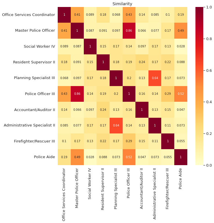
../_images/128b4d668af3f4ba5dd4214e921d6d6ee1564d41922293dc374d2c0ea9fdf6f2.png

As we can see from the matrix above,

The similarity between the same strings such as ‘Office Services Coordinator’ and ‘Office Services Coordinator’ is 1
The similarity between somewhat similar strings such as ‘Office Services Coordinator’ and ‘Master Police Officer’ is 0.41
The similarity between two very different strings such as ‘Social Worker IV’ and ‘Polic Aide’ is 0.028

Link to dirty-cat.

Link to my full article about dirty-cat.

6.2.11. How to Handle Misspellings in Real-World Datasets#

Real-world datasets often contain misspellings, particularly in manually entered categorical variables.

To merge multiple variants of the same category, use skub’s deduplicate function, which:

Measures the distance between strings and groups similar strings together
Replaces the strings in each group with the most common string

To demonstrate the deduplicate function, start with generating a duplicated dataset:

from skrub.datasets import make_deduplication_data
import pandas as pd

duplicated_food = make_deduplication_data(
    examples=["Chocolate", "Broccoli", 'Jalapeno', 'Zucchini'],  
    entries_per_example=[100, 200, 300, 200],  # their respective number of occurrences
    prob_mistake_per_letter=0.05,  # 5% probability of typo per letter
    random_state=42,  # set seed for reproducibility
)

duplicated_food[:5]

['Chocolate', 'Cgocolate', 'Chocolate', 'Chqcolate', 'Chocoltte']

Get the most common food names:

import collections
counter = collections.Counter(duplicated_food)
counter.most_common(20)

[('Jalapeno', 284),
 ('Zucchini', 195),
 ('Broccoli', 193),
 ('Chocolate', 94),
 ('Jalaoeno', 2),
 ('Cgocolate', 1),
 ('Chqcolate', 1),
 ('Chocoltte', 1),
 ('Chocdlate', 1),
 ('ehocolate', 1),
 ('Chocolatw', 1),
 ('Brocroli', 1),
 ('Brojcoli', 1),
 ('Broccsli', 1),
 ('Broccqli', 1),
 ('Bxoccoli', 1),
 ('sroccoli', 1),
 ('Brzccoli', 1),
 ('Jylapeno', 1),
 ('Jalapony', 1)]

The most common words in the dataset are ‘Jalapeno’, ‘Zucchini’, and ‘Broccoli’. Therefore, skub’s deduplicate function replaces misspelled words with the closest matching word from this set.

from skrub import deduplicate

deduplicated_data = deduplicate(duplicated_food)

counter = collections.Counter(deduplicated_data)
counter.items()

dict_items([('Chocolate', 100), ('Broccoli', 200), ('Jalapeno', 300), ('Zucchini', 200)])

# create a table that maps original to corrected categories
translation_table = pd.Series(deduplicated_data, index=duplicated_food)

# remove duplicates in the original data
translation_table = translation_table[~translation_table.index.duplicated(keep="first")]

translation_table.sample(10)

Brojcoli      Broccoli
qalapeno      Jalapeno
Jalapenh      Jalapeno
Jalapeto      Jalapeno
Zucchini      Zucchini
oalapeno      Jalapeno
Bxoccoli      Broccoli
Jalqceno      Jalapeno
Jzlapeno      Jalapeno
ehocolate    Chocolate
dtype: object

Link to skub.

6.2.12. Solving Data Mismatches: Joining Tables with Fuzzy Matching#

Frequently, entries in one table may not have an exact match in another table. For instance, one table might have “Yemen*” while the other has “Yemen, Rep.”

The fuzzy_join() function in skrub enables joining tables without the need for extensive data cleaning by accounting for the label variations.

import pandas as pd

df = pd.read_csv(
    "https://raw.githubusercontent.com/skrub-data/datasets/master/data/Happiness_report_2022.csv",
    thousands=",",
)
df = df[["Country", "Happiness score"]]

from skrub.datasets import fetch_world_bank_indicator
gdppc = fetch_world_bank_indicator(indicator_id="NY.GDP.PCAP.CD").X

print(df.sort_values(by="Country").tail(6))

       Country  Happiness score
Venezuela           4925.0
   Vietnam           5485.0
   Yemen*           4197.0
   Zambia           3760.0
 Zimbabwe           2995.0
       xx              NaN

print(gdppc.sort_values(by="Country Name").tail(5))

           Country Name  GDP per capita (current US$)
West Bank and Gaza                   3789.327966
             World                  12647.480789
       Yemen, Rep.                    701.714878
            Zambia                   1487.907764
          Zimbabwe                   1266.996031

from skrub import fuzzy_join

df1 = fuzzy_join(
    df,  # our table to join
    gdppc,  # the table to join with
    left_on="Country",  # the first join key column
    right_on="Country Name",  # the second join key column
    return_score=True,
)

print(df1[['Country', 'Country Name', "matching_score"]].tail(20))
# We merged the first WB table to our initial one.

          Country                                 Country Name  matching_score
 Madagascar*                                   Madagascar        0.795045
       Egypt                             Egypt, Arab Rep.        0.654033
       Chad*                                         Chad        0.683373
    Ethiopia                                     Ethiopia        1.000000
      Yemen*                                  Yemen, Rep.        0.653668
 Mauritania*                                   Mauritania        0.810736
      Jordan                                       Jordan        1.000000
        Togo                                         Togo        1.000000
       India                                        India        1.000000
      Zambia                                       Zambia        1.000000
      Malawi                                       Malawi        1.000000
    Tanzania                                     Tanzania        1.000000
Sierra Leone                                 Sierra Leone        1.000000
    Lesotho*                                      Lesotho        0.755238
   Botswana*                                     Botswana        0.795825
     Rwanda*                                       Rwanda        0.754604
    Zimbabwe                                     Zimbabwe        1.000000
     Lebanon                                      Lebanon        1.000000
 Afghanistan                                  Afghanistan        1.000000
          xx  East Asia & Pacific (excluding high income)        0.500000

Link to skrub.

6.2.13. Snorkel — Programmatically Build Training Data in Python#

Imagine you try to determine whether a job posting is fake or not. You come up with some assumptions about a fake job posting, such as:

If a job posting has few to no descriptions about the requirements, it is likely to be fake.
If a job posting does not include any company profile or logo, it is likely to be fake.
If the job posting requires some sort of education or experience, it is likely to be real.

import pandas as pd 
import warnings
warnings.simplefilter(action='ignore', category=FutureWarning)


train_df = pd.read_pickle(
    "https://github.com/khuyentran1401/Data-science/blob/master/feature_engineering/snorkel_example/train_fake_jobs.pkl?raw=true"
)
train_df.head(5)

	job_id	title	location	department	salary_range	company_profile	description	requirements	benefits	has_company_logo	has_questions	employment_type	required_experience	required_education	industry	function
12276	12277	Big Data Analyst	GB, WSM, London	Product Ops	NaN	Founded in 2010 by a team from Google’s London...	Qubit: Cutting Edge Big Data EngineeringQubit ...	What you'll need: A background in consulting, ...	Plenty of perks:As well as the opportunity to ...	1	1	Full-time	Associate	Bachelor's Degree	Internet	Product Management
14680	14681	Instructional Advocate	US, GA, Savannah	NaN	NaN	We are an after-school program committed to as...	21st Century Community Learning Centers is an ...	Bachelor's Degree or an Associate's Degree; or...	NaN	1	0	Part-time	NaN	NaN	NaN	Education
16518	16519	Software Developer	US, FL, Gainesville	NaN	NaN	352 Inc. is a full-service digital agency crea...	We partner with great clients to build smart s...	3-5 years of great c# work Experience in mvc o...	What You’ll GetFreedom: We trust you to do you...	1	0	Full-time	Mid-Senior level	NaN	Computer Software	Information Technology
15478	15479	Internship in India	IN, , Bangalore	NaN	NaN		London is a fast paced city of culture, divers...		As specialists in delivering high quality and ...	1	0	NaN	NaN	NaN	NaN	NaN
16348	16349	Web Developer Backend Microservices (m/f)	DE, BE, 10969	Engineering	NaN	airfy prägt sicheres und einfach zu bedienende...	Design and develop a microservice platform for...	Senior level experience with web backends, esp...	Flat hierarchies and a productive work environ...	1	0	Full-time	Associate	Bachelor's Degree	Internet	Engineering

How do you test which of these features are the most accurate in predicting fraud?

That is when Snorkel comes in handy. Snorkel is an open-source Python library for programmatically building training datasets without manual labeling.

To learn how Snorkel works, start with giving a meaningful name to each value:

from snorkel.labeling import labeling_function, PandasLFApplier, LFAnalysis

FAKE = 1
REAL = 0
ABSTAIN = -1

We assume that:

Fake companies don’t have company profiles or logos
Fake companies are found in a lot of fake job postings
Real job postings often requires a certain level of experience and education

Let’s test those assumptions using Snorkel’s labeling_function decorator. The labeling_function decorator allows us to quickly label instances in a dataset using functions.

@labeling_function()
def no_company_profile(x: pd.Series):
    return FAKE if x.company_profile == "" else ABSTAIN


@labeling_function()
def no_company_logo(x: pd.Series):
    return FAKE if x.has_company_logo == 0 else ABSTAIN


@labeling_function()
def required_experience(x: pd.Series):
    return REAL if x.required_experience else ABSTAIN


@labeling_function()
def required_education(x: pd.Series):
    return REAL if x.required_education else ABSTAIN

ABSTAIN or -1 tells Snorkel not to make any conclusion about the instance that doesn’t satisfy the condition.

Next, we will use each of these labeling functions to label our training dataset:

lfs = [
    no_company_profile,
    no_company_logo,
    required_experience,
    required_education,
]

applier = PandasLFApplier(lfs=lfs)
L_train = applier.apply(df=train_df)

100%|██████████████████████████████████████████████| 13410/13410 [00:02<00:00, 5849.25it/s]

Now that we have created the labels using each labeling function, we can use LFAnalysis to determine the accuracy of these labels.

LFAnalysis(L=L_train, lfs=lfs).lf_summary(Y=train_df.fraudulent.values)

	j	Polarity	Coverage	Overlaps	Conflicts	Correct	Incorrect	Emp. Acc.
no_company_profile	0	[1]	0.186204	0.186204	0.186204	459	2038	0.183821
no_company_logo	1	[1]	0.205742	0.205742	0.205742	459	2300	0.166365
required_experience	2	[0]	1.000000	1.000000	0.244295	12741	669	0.950112
required_education	3	[0]	1.000000	1.000000	0.244295	12741	669	0.950112

Details of the statistics in the table above:

Polarity: The set of unique labels this LF outputs (excluding abstains)
Coverage: The fraction of the dataset that is labeled
Overlaps: The fraction of the dataset where this LF and at least one other LF agree
Conflicts: The fraction of the dataset where this LF and at least one other LF disagree
Correct: The number of data points this LF labels correctly
Incorrect: The number of data points this LF labels incorrectly
Empirical Accuracy: The empirical accuracy of this LF

Link to Snorkel.

My full article about Snorkel.

6.2.14. sketch: AI Code-Writing Assistant That Understands Data Content#

Wouldn’t it be nice if you could get insights into your data by simply asking a question? Sketch allows you to do exactly that.

Sketch is an AI code-writing assistant for pandas users that understands the context of your data.

import pandas as pd  
import seaborn as sns 
import sketch

data = sns.load_dataset('taxis')
data.head(10)

	pickup	dropoff	passengers	distance	fare	tip	total	color	payment	pickup_zone	dropoff_zone	pickup_borough	dropoff_borough
0	2019-03-23 20:21:09	2019-03-23 20:27:24	1	1.60	7.0	2.15	12.95	yellow	credit card	Lenox Hill West	UN/Turtle Bay South	Manhattan	Manhattan
1	2019-03-04 16:11:55	2019-03-04 16:19:00	1	0.79	5.0	0.00	9.30	yellow	cash	Upper West Side South	Upper West Side South	Manhattan	Manhattan
2	2019-03-27 17:53:01	2019-03-27 18:00:25	1	1.37	7.5	2.36	14.16	yellow	credit card	Alphabet City	West Village	Manhattan	Manhattan
3	2019-03-10 01:23:59	2019-03-10 01:49:51	1	7.70	27.0	6.15	36.95	yellow	credit card	Hudson Sq	Yorkville West	Manhattan	Manhattan
4	2019-03-30 13:27:42	2019-03-30 13:37:14	3	2.16	9.0	1.10	13.40	yellow	credit card	Midtown East	Yorkville West	Manhattan	Manhattan
5	2019-03-11 10:37:23	2019-03-11 10:47:31	1	0.49	7.5	2.16	12.96	yellow	credit card	Times Sq/Theatre District	Midtown East	Manhattan	Manhattan
6	2019-03-26 21:07:31	2019-03-26 21:17:29	1	3.65	13.0	2.00	18.80	yellow	credit card	Battery Park City	Two Bridges/Seward Park	Manhattan	Manhattan
7	2019-03-22 12:47:13	2019-03-22 12:58:17	0	1.40	8.5	0.00	11.80	yellow	NaN	Murray Hill	Flatiron	Manhattan	Manhattan
8	2019-03-23 11:48:50	2019-03-23 12:06:14	1	3.63	15.0	1.00	19.30	yellow	credit card	East Harlem South	Midtown Center	Manhattan	Manhattan
9	2019-03-08 16:18:37	2019-03-08 16:26:57	1	1.52	8.0	1.00	13.30	yellow	credit card	Lincoln Square East	Central Park	Manhattan	Manhattan

data.sketch.ask(
    "Can you give me friendly names for each column?" 
    "(Output as an HTML list)"
)

Index: Row Number
Pickup: Pickup Time
Dropoff: Dropoff Time
Passengers: Number of Passengers
Distance: Distance Travelled
Fare: Fare Amount
Tip: Tip Amount
Tolls: Tolls Amount
Total: Total Amount
Color: Vehicle Color
Payment: Payment Method
Pickup Zone: Pickup Zone Name
Dropoff Zone: Dropoff Zone Name
Pickup Borough: Pickup Borough Name
Dropoff Borough: Dropoff Borough Name

data.sketch.ask(
    "Which payment is the most popular payment?"
)

The most popular payment is credit card.

data.sketch.howto("Create some features from the pickup column")

# Create a new column for the hour of the pickup
data['pickup_hour'] = data['pickup'].dt.hour

# Create a new column for the day of the week of the pickup
data['pickup_day'] = data['pickup'].dt.weekday_name

# Create a new column for the month of the pickup
data['pickup_month'] = data['pickup'].dt.month_name()

# Create a new column for the hour of the pickup
data['pickup_hour'] = data['pickup'].dt.hour

# Create a new column for the day of the week of the pickup
data['pickup_day'] = data['pickup'].dt.weekday

# Create a new column for the month of the pickup
data['pickup_month'] = data['pickup'].dt.month_name()

data.sketch.howto(
    "Create some features from the pickup_zone column"
)

# Create a new column called 'pickup_zone_count'
data['pickup_zone_count'] = data.groupby('pickup_zone')['pickup_zone'].transform('count')

# Create a new column called 'pickup_zone_fare'
data['pickup_zone_fare'] = data.groupby('pickup_zone')['fare'].transform('mean')

# Create a new column called 'pickup_zone_distance'
data['pickup_zone_distance'] = data.groupby('pickup_zone')['distance'].transform('mean')

# Create a new column called 'pickup_zone_count'
data['pickup_zone_count'] = data.groupby('pickup_zone')['pickup_zone'].transform('count')

# Create a new column called 'pickup_zone_fare'
data['pickup_zone_fare'] = data.groupby('pickup_zone')['fare'].transform('mean')

# Create a new column called 'pickup_zone_distance'
data['pickup_zone_distance'] = data.groupby('pickup_zone')['distance'].transform('mean')

data

	pickup	dropoff	passengers	distance	fare	tip	tolls	total	color	payment	pickup_zone	dropoff_zone	pickup_borough	dropoff_borough	pickup_hour	pickup_day	pickup_month	pickup_zone_count	pickup_zone_fare	pickup_zone_distance
0	2019-03-23 20:21:09	2019-03-23 20:27:24	1	1.60	7.0	2.15	0.0	12.95	yellow	credit card	Lenox Hill West	UN/Turtle Bay South	Manhattan	Manhattan	20	5	March	120.0	9.016667	1.857083
1	2019-03-04 16:11:55	2019-03-04 16:19:00	1	0.79	5.0	0.00	0.0	9.30	yellow	cash	Upper West Side South	Upper West Side South	Manhattan	Manhattan	16	0	March	144.0	9.987778	2.031597
2	2019-03-27 17:53:01	2019-03-27 18:00:25	1	1.37	7.5	2.36	0.0	14.16	yellow	credit card	Alphabet City	West Village	Manhattan	Manhattan	17	2	March	9.0	11.944444	2.796667
3	2019-03-10 01:23:59	2019-03-10 01:49:51	1	7.70	27.0	6.15	0.0	36.95	yellow	credit card	Hudson Sq	Yorkville West	Manhattan	Manhattan	1	6	March	47.0	11.000000	2.243830
4	2019-03-30 13:27:42	2019-03-30 13:37:14	3	2.16	9.0	1.10	0.0	13.40	yellow	credit card	Midtown East	Yorkville West	Manhattan	Manhattan	13	5	March	198.0	10.994949	2.239798
...	...	...	...	...	...	...	...	...	...	...	...	...	...	...	...	...	...	...	...	...
6428	2019-03-31 09:51:53	2019-03-31 09:55:27	1	0.75	4.5	1.06	0.0	6.36	green	credit card	East Harlem North	Central Harlem North	Manhattan	Manhattan	9	6	March	72.0	12.550000	2.854306
6429	2019-03-31 17:38:00	2019-03-31 18:34:23	1	18.74	58.0	0.00	0.0	58.80	green	credit card	Jamaica	East Concourse/Concourse Village	Queens	Bronx	17	6	March	12.0	25.597500	7.261667
6430	2019-03-23 22:55:18	2019-03-23 23:14:25	1	4.14	16.0	0.00	0.0	17.30	green	cash	Crown Heights North	Bushwick North	Brooklyn	Brooklyn	22	5	March	12.0	14.549167	3.665000
6431	2019-03-04 10:09:25	2019-03-04 10:14:29	1	1.12	6.0	0.00	0.0	6.80	green	credit card	East New York	East Flatbush/Remsen Village	Brooklyn	Brooklyn	10	0	March	10.0	32.409000	7.086000
6432	2019-03-13 19:31:22	2019-03-13 19:48:02	1	3.85	15.0	3.36	0.0	20.16	green	credit card	Boerum Hill	Windsor Terrace	Brooklyn	Brooklyn	19	2	March	21.0	11.761905	2.812857

6433 rows × 20 columns

Link to sketch.

Feature Engineer

Contents

6.2. Feature Engineer#

6.2.1. Split Data in a Stratified Fashion in scikit-learn#

6.2.2. Strategy to Prevent Data Leakage in Time-correlated Datasets#

6.2.3. Enhancing Data Handling with scikit-learn’s DataFrame Support#

6.2.4. Efficient Feature Transformation with make_column_transformer in scikit-learn#

6.2.5. FunctionTransformer: Build Robust Preprocessing Pipelines with Custom Transformations#

6.2.6. Drop Correlated Features#

6.2.7. Encode Rare Labels with Feature-engine#

6.2.8. Encode Categorical Data Using Frequency#

6.2.9. Return a DataFrame When Using a scikit-learn’s Transformer#

6.2.10. Similarity Encoding for Dirty Categories Using dirty_cat#

6.2.11. How to Handle Misspellings in Real-World Datasets#

6.2.12. Solving Data Mismatches: Joining Tables with Fuzzy Matching#

6.2.13. Snorkel — Programmatically Build Training Data in Python#

6.2.14. sketch: AI Code-Writing Assistant That Understands Data Content#